For loops vs. apply - a race in efficiency
#projects #rWritten by Matt Sosna on July 13, 2017
Welcome to the first Random R post, where we ask random programming questions and use R to figure them out. In this post we’ll look at the computational efficiency of for loops versus the apply function.
Background
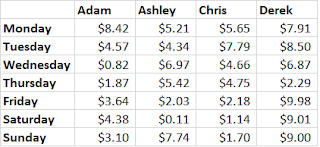
for loops are a way of executing a command again and again, with one (or more) variable value changed each time. Let’s say we have data on a bunch of people for food-related spending over one week. (And that yes, some days they spent only $0.11 and they never spent more than $10. Bear with me.) The first four columns of our matrix look like this:

If we want to know the average amount each person spent that week, we can take the mean of every column. If our matrix is called our_matrix, we could type out:
| R |
1
2
3
4
5
mean(our_matrix[, 1])
mean(our_matrix[, 2])
mean(our_matrix[, 3])
mean(our_matrix[, 4])
...
But a simpler way to do this, especially if you have a lot of columns, would be to iterate through the columns with a for loop, like this:
| R |
1
2
3
for(i in 1:ncol(our_matrix)){
   mean(our_matrix[, i])
}
Here, the value of i is being replaced with the number 1, 2, 3, etc. up to the matrix’s number of columns.
Conceptually, this is pretty easy to understand. for loops are straightforward and for many applications, they’re an excellent way to get stuff done. (We’ll use nested loops in the next section, for example.) But one of the first things a beginning coder might hear about for loops is that as soon as you get the hang of them, it’s a good idea to move onto more elegant functions that are simpler and faster. (This DataCamp intro to loops post, for example, mentions alternatives in the same sentence it introduces for loops!) One such “elegant” command is called apply.
| R |
1
apply(our_matrix, 2, mean)
The apply command above does the same thing as the two preceding chunks of code, but it’s much shorter and considered better practice to use. We’re making our final script length shorter and the code above is easier to read. But what about what’s going on under the hood? Does your computer find the above command actually faster to compute? Let’s find out.
Methods
At its core, our methods will involve:
- Creating a matrix
- Performing a calculation on every column in the matrix with either a
forloop orapply - Timing how long the process took
We’ll then compare the computation times, which will be our measure of efficiency. Before we get started, however, we’ll address three additional points:
1. Examine the role of matrix size
If there are differences in computational efficiency between for loops and apply, the differences will be more pronounced for larger matrices. In other words, if you want to know if you or your girlfriend is a better endurance runner, you’ll get a more accurate answer if you run a marathon than if you race to that plate of Nachos on the table. (Save yourself an argument about fast-twitch versus slow-twitch muscle and just agree that watching Michael Phelps YouTube videos basically counts as exercise anyway.) So as we pit our competing methods against each other, we want to give them a task that will maximize the difference in their effectiveness.
But the nice thing about coding is that it’s often really easy to get a more nuanced answer to our question with just a few more lines of code. So let’s ask how the difference in effectiveness between for loops and apply changes with the size of the matrix. Maybe there’s effectively no difference until you’re dealing with matrices the size of what Facebook knows about your personal life, or maybe there are differences in efficiency right from the start. To look at this, we’ll keep the number of columns constant at 1,000 but we’ll vary the size of each column from 2 rows to 1,000.
2. Vary how difficult the computation is
Maybe our results will depend on what computation, exactly, we’re performing on our matrices. We’ll use a simple computation (just finding the mean) and a more complicated one (finding the mean of the six smallest values, which requires sorting and subsetting too).
3. Minimize the role of chance
At the core of statistics is that there are innumerable random forces swaying the results in any data collection we perform. Maybe that bird preening itself just had an itch and isn’t actually exhibiting some complex self recognition. Maybe the person misread the survey question and doesn’t actually think the capital of Montana is the sun. One way we address this randomness we can’t control for is through replication. We give a survey to lots of people; we look at lots of birds. One sun-lover is probably a mistake, but if everyone in the survey thought the sun was the capital, then we need to sit down and reevaluate where people think Montana is. So in our code, we’ll run our simulation 10 times to account for randomness within our computer’s processing time.
[The code to carry out these ideas is at the bottom of the post. Otherwise, let’s look at some figures.]
Results
1. Simple calculation

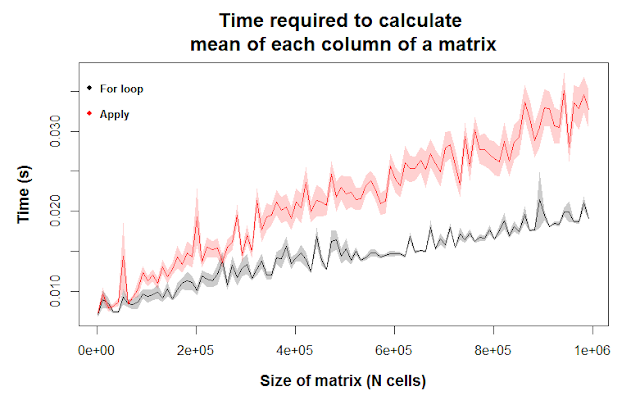
In the figure above, the gray and red colors correspond to for loops and apply, respectively. The lines are the mean values for 10 runs, and the shaded regions are the means \(\pm\) 1 standard error. [Note that if we want to comment on statistical significance, we’d have to multiply the standard errors by 1.96 to get 95% confidence intervals. If those envelopes didn’t overlap, we could then be confident that the differences we see are statistically significant. I didn’t do that in this post, but you should keep that in mind.]
The y-axis corresponds to the time it took to perform the calculation. Lower values means the calculation was faster. As you move to the right on the x-axis, you’re seeing the computational time for increasingly larger matrices. We see the gray and red lines diverge because the differences in computational efficiency grow larger as we give R an increasingly difficult task. For relatively small matrices, though, there’s essentially no difference in computational efficiency between the two methods.
In summary, we have evidence that for loops outcompete apply for a simple task on matrices above roughly 300,000 cells. Below that size, though (which is pretty big), you won’t see any difference in how fast the calculation is run. Even for a matrix with a million data points, an average laptop can find the mean of each column in less than 1/20 of a second.
2. More complex calculation
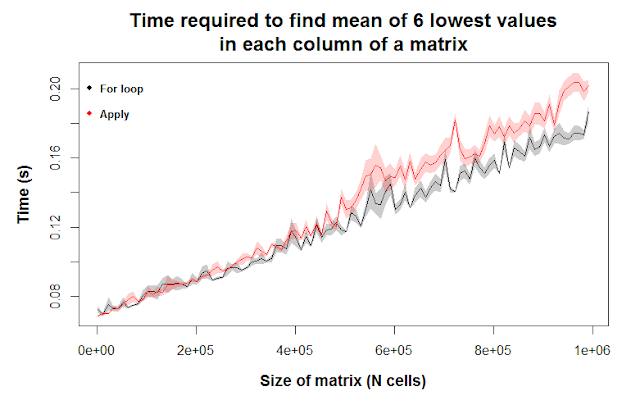
Here, we’re asking R to find the mean of the six lowest values of each column of a matrix. This requires R to first order the column values from smallest to largest, then isolate the smallest six values, then take the mean of those values. According to our figure, we find any differences between for loops and apply to be negligible.

Maybe for incredibly large matrices, for loops are slightly more efficient, as seen by the shaded regions not overlapping at the far right of the figure. However, we should still be careful in interpreting this figure; while the error envelopes don’t overlap for some matrix sizes (e.g. ~720k cells, 1 million), they do for other matrix sizes (e.g. 600k, 825k), meaning the differences we’re seeing are likely due to chance.
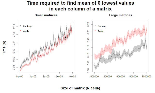
Ten replicates of our simulation is clearly not enough to reject the idea that there’s any difference between for loops and the apply function here. Let’s rerun the code with more replicates. To save time, we’ll focus on small and large matrices and skip intermediate sizes.

With the additional clarity of 50 replicates, we can see that for very small matrices, apply appears to outperform for loops. Any differences quickly become negligible as we increase matrix size. For large matrices, we see a fairly consistent superiority of for loops when the matrices are greater than 900,000 cells, meaning our original intuition seems to hold. This indicates that for loops are more efficient at performing this complicated function than apply, but only when the matrices are huge. Meanwhile, apply might actually be stronger for relatively small matrices, which many users are more likely to be dealing with.
Discussion
So we see that for loops often have a slight edge over apply in terms of speed, especially for simple calculations or on huge matrices. Cool, but this leaves us with a few questions.
Why are for loops more efficient?
The results above came as a surprise to me because I’d always heard about how inefficient for loops can be. It turns out I’d missed the bit that should follow that statement: for loops can be inefficient, but not if your code allocates memory well. A massively inefficient way to write a for loop is to have a variable that you overwrite with every iteration, e.g. vec <- c(vec, new_value). That basically forces R to recall the result of every previous iteration, for every iteration. If you look at the code at the end of the post, you’ll see that we instead created empty matrices whose cells were filled with values.
So we didn’t mess up, but that doesn’t fully explain why for loops are faster. According to this thread on Stack Exchange, a for loop can outcompete apply here because for loops use the vectorized indexes of a matrix, while apply converts each row into a vector, performs the calculations, and then has to convert the results back into an output.
[For those of you who are really into the technical details, lapply is an exception and is actually faster than for loops because more of its calculations are brought down into the language C and performed there.]
If for loops are generally faster, why bother with apply?
The figures in this post have shown that apply is usually a bit slower than for loops. But does a difference of 0.01 seconds, or even 0.1 seconds, matter? If you’re performing an evolutionary simulation on huge populations for thousands of generations, and you’re doing this multiple times with different model parameters… then sure, those 0.1 seconds will add up. But outside of such a computation-heavy scenario (where you’re better off moving your code out of R and into C or C++, anyway), the clarity in reading apply commands is far more important, I would argue. If you’re sharing your code with a collaborator, or writing code you might read again in the future, you want to be as clear as possible. Concise code is better than a sprawling mess.
Thanks for reading. If you have any suggestions for a fun R project, shoot me an e-mail.
Best,
Matt
Code for this post
[Note: I’m just including the code for the complicated calculation. For the simple calculation, replace mean(head(sort(data[, k]))) with mean(data[,k]) in the nested for loop.]
| R |
1
2
3
4
5
6
7
8
9
10
11
12
13
14
15
16
17
18
19
20
21
22
23
24
25
26
27
28
29
30
31
32
33
34
35
36
37
38
39
40
41
42
43
44
45
46
47
48
49
50
51
52
53
54
55
56
57
58
59
60
61
62
63
64
65
66
67
68
69
70
71
# Set N reps and range in matrix sizes
replicates <- 10
n.rows <- seq(2, 1000, by = 10)  # Range in matrix sizes

# Initialize matrices to fill
loop.times <- matrix(NA, nrow = replicates, ncol = length(n.rows))
apply.times <- matrix(NA, nrow = replicates, ncol = length(n.rows))

# Run the analysis
for(i in 1:replicates){
  for(j in 1:length(n.rows)){
     data <- matrix(rnorm(1000 * n.rows[j]),
                    ncol = 1000, nrow = n.rows[j])

     # Method 1: for loop
     start.time <- Sys.time()
     for(k in 1:ncol(data)){
       mean(head(sort(data[, k])))
     }
     loop.times[i, j] <- difftime(Sys.time(), start.time)

     # Method 2: apply
     start.time <- Sys.time()
     apply(data, 2, function(x){mean(head(sort(x)))})
     apply.times[i, j] <- difftime(Sys.time(), start.time)

   print(paste0("Replicate ", i, "| iteration ", j))
  }
}

# Prepare for plotting
size <- n.rows * 1000

# Get the mean times and SE for loops versus apply
m.loop <- apply(loop.times, 2, mean)
se.loop <- apply(loop.times, 2, sd) / sqrt(replicates)

m.apply <- apply(apply.times, 2, mean)
se.apply <- apply(apply.times, 2, sd) / sqrt(replicates)

# Create the error envelopes. Note that the x-coordinate is the same
coord.x <- c(size, size[length(size)], rev(size))
coord.y.loop <- c(m.loop + se.loop,
                  m.loop[length(m.loop)] - se.loop[length(se.loop)],
                  rev(m.loop - se.loop))

coord.y.apply <- c(m.apply + se.apply,
                   m.apply[length(m.apply)] - se.apply[length(se.apply)],
                   rev(m.apply - se.apply))

# Plot it
# 1st: plot the mean loop times
plot(size, m.loop, type = 'l',
     ylim = c(min(m.loop - se.loop), max(m.apply + se.apply)),
     main = "Time required to find mean of 6 lowest values
in each column of a matrix",
     xlab = "Size of matrix (N cells)", ylab = "Time (s)",
     cex.main = 1.5, cex.lab = 1.2, font.lab = 2)

# Add the error envelope
polygon(coord.x, coord.y.loop, col = "gray80", border = NA)
lines(size, m.loop)

# Add the mean apply times
lines(size, m.apply, col = "red")
polygon(coord.x, c.y.apply, col = rgb(1, 0.1, 0.1, 0.2), border = NA)

# Add the legend
par(font = 2)
legend("topleft", col = 1:2, pch = 19, cex = 0.8,
       c("For loop", "Apply"), bty = 'n')
