
Building a Random Forest by Hand in Python
#machine-learningWritten by Matt Sosna on January 28, 2024
From drug discovery to species classification, credit scoring to cybersecurity and more, the random forest is a popular and powerful algorithm for modeling our complex world. Its versatility and predictive prowess would seem to require cutting-edge complexity, but if we dig into what a random forest actually is, we see a shockingly simple set of repeating steps.
I find that the best way to learn something is to play with it. So to gain an intuition on how random forests work, let’s build one by hand in Python, starting with a decision tree and expanding to the full forest. We’ll see first-hand how flexible and interpretable this algorithm is for both classification and regression. And while this project may sound complicated, there are really only a few core concepts we’ll need to learn: 1) how to iteratively partition data, and 2) how to quantify how well data is partitioned.
Background
Decision tree inference
A decision tree is a supervised learning algorithm that identifies a branching set of binary rules that map features to labels in a dataset. Unlike algorithms like logistic regression where the output is an equation, the decision tree algorithm is nonparametric, meaning it doesn’t make strong assumptions on the relationship between features and labels. This means that decision trees are free to grow in whatever way best partitions their training data, so the resulting structure will vary between datasets.
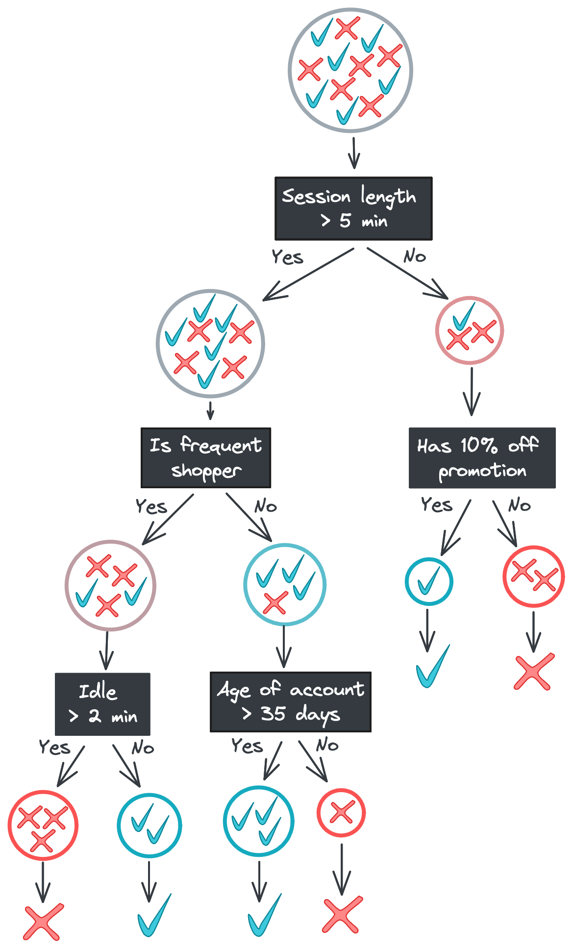
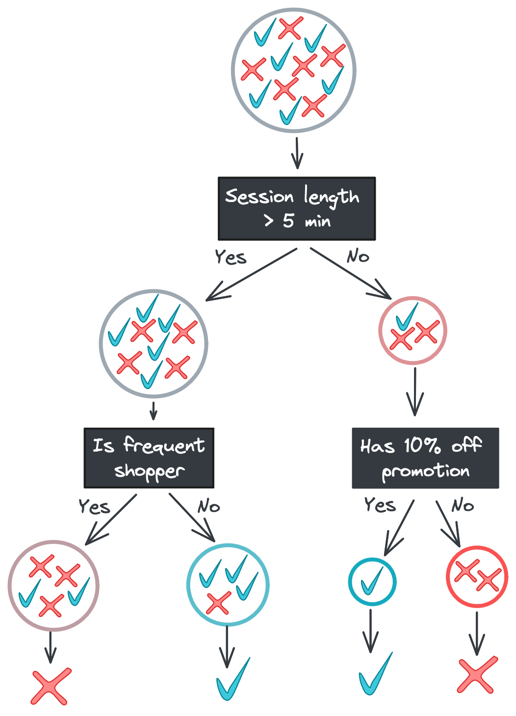
One major benefit of decision trees is their explainability: each step the tree takes in deciding how to predict a category (for classification) or continuous value (for regression) can be seen in the tree nodes. A model that predicts whether a shopper will buy a product they viewed online, for example, might look like this.
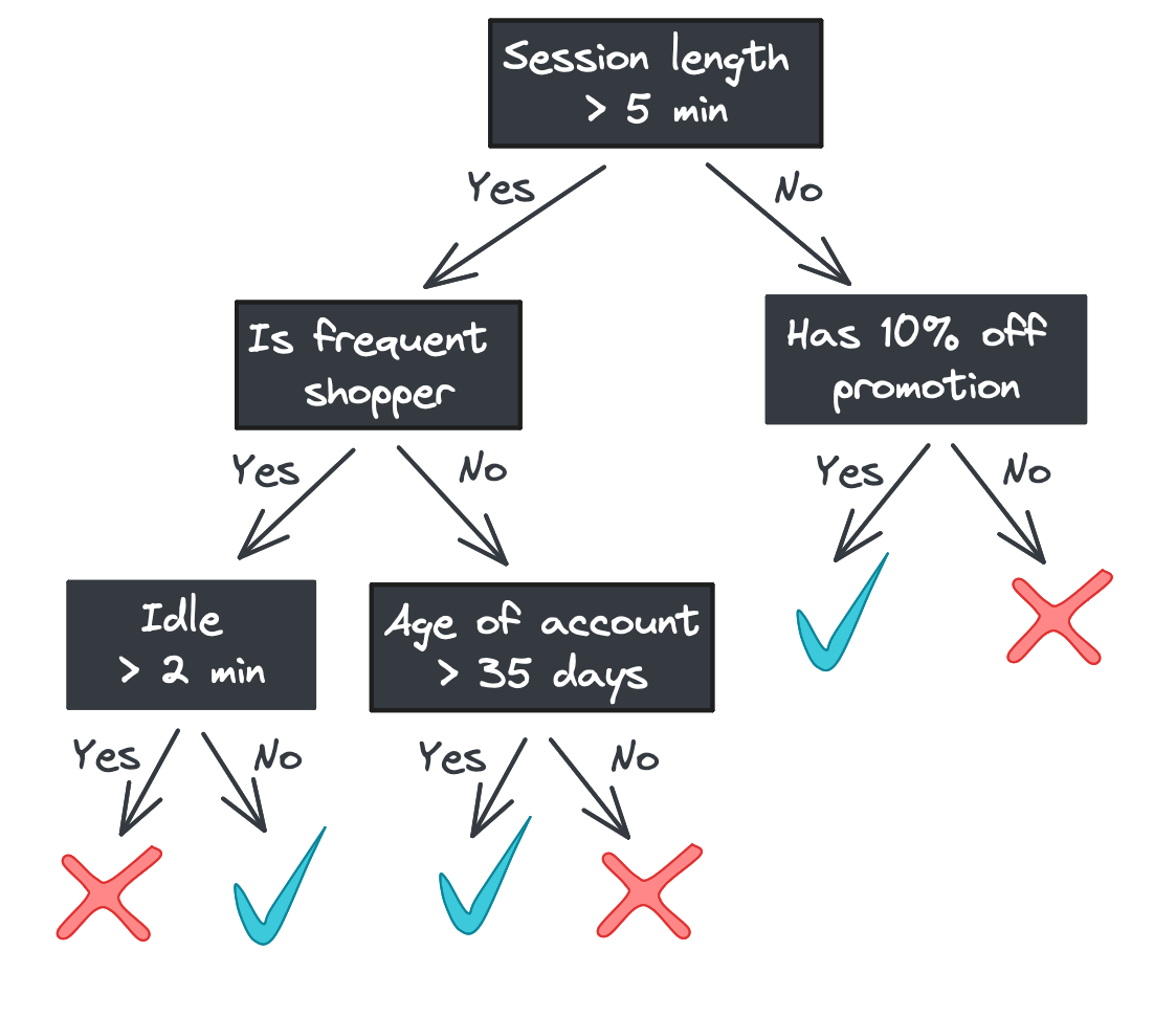
Starting with the root, each node in the tree asks a binary question (e.g., “Was the session length longer than 5 minutes?”) and passes the feature vector to one of two child nodes depending on the answer. If there are no children – i.e., we’re at a leaf node – then the tree returns a response.

(We’ll focus on classification in this blog post, but a decision tree regressor would look identical but with continuous values returned rather than class labels.)
Decision tree training
Inference, or this prediction process, is pretty straightforward. But building this tree is much less obvious. How is the binary rule in each node determined? Which features are used in the tree, and in what order? Where does a threshold like 0.5 or 1 come from?
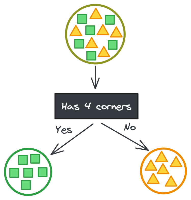
To understand how decision trees are built, let’s imagine we’re trying to partition a large dataset of shapes (squares and triangles) into smaller datasets of only squares or only triangles based on their features. In the ideal case, there’s some categorical feature that perfectly separates the shapes.
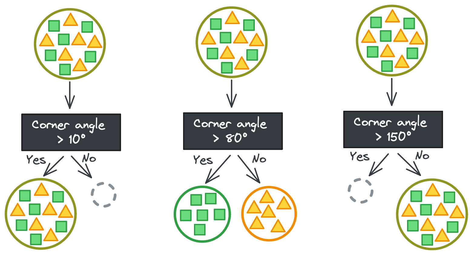
But it’s never that easy. If you’re lucky, maybe there’s a continuous feature that has some threshold that perfectly separates the shapes instead. It takes a couple tries to find the exact threshold, but then you have your perfect split. (Phew!)
Well… it’s never really that easy, either. In this toy example, all triangles and squares are identical, meaning it’s trivial to separate their feature vectors. (Find one rule that works for one triangle and it works for all triangles!)
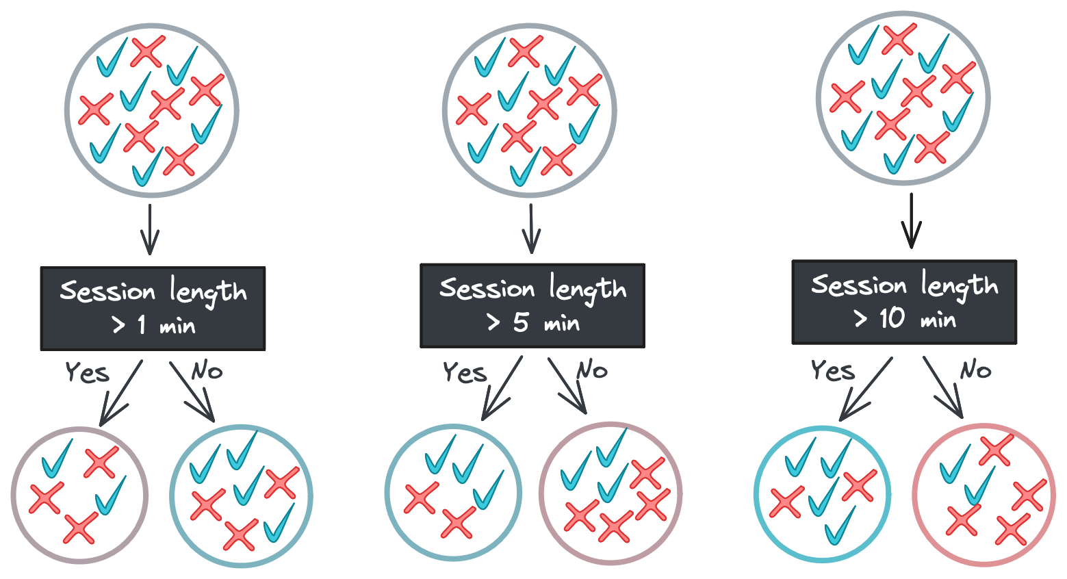
But in the real world, features don’t map so neatly to labels. Going back to our e-commerce example, a feature like time spent on the site in a session might not be able to perfectly partition the classes at any threshold.
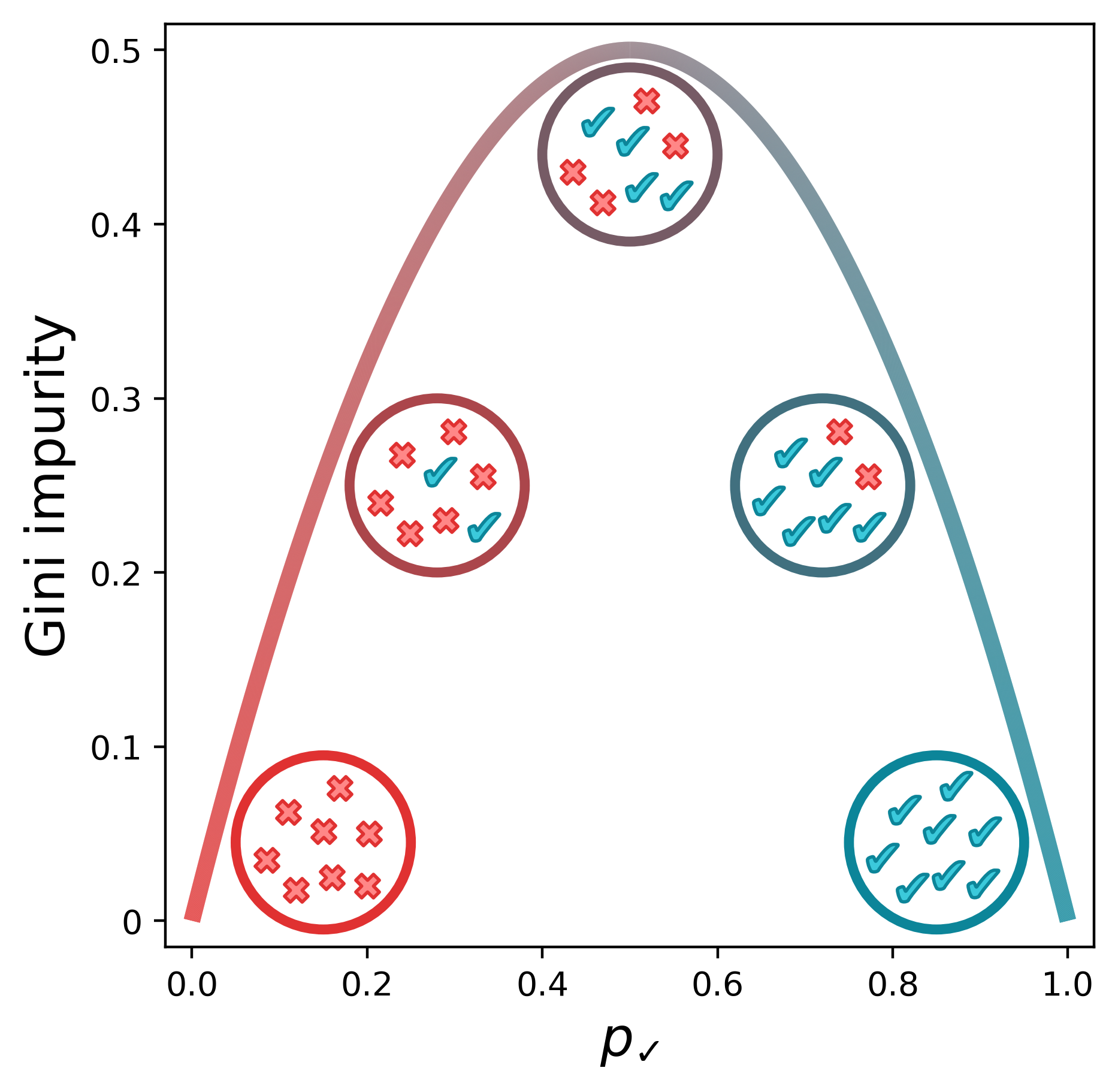
So what do we do if no feature at any threshold can perfectly split our data? In this case, we need a way to quantify how “mixed” a set of labels is. One common metric is Gini impurity, which is calculated with the following equation:
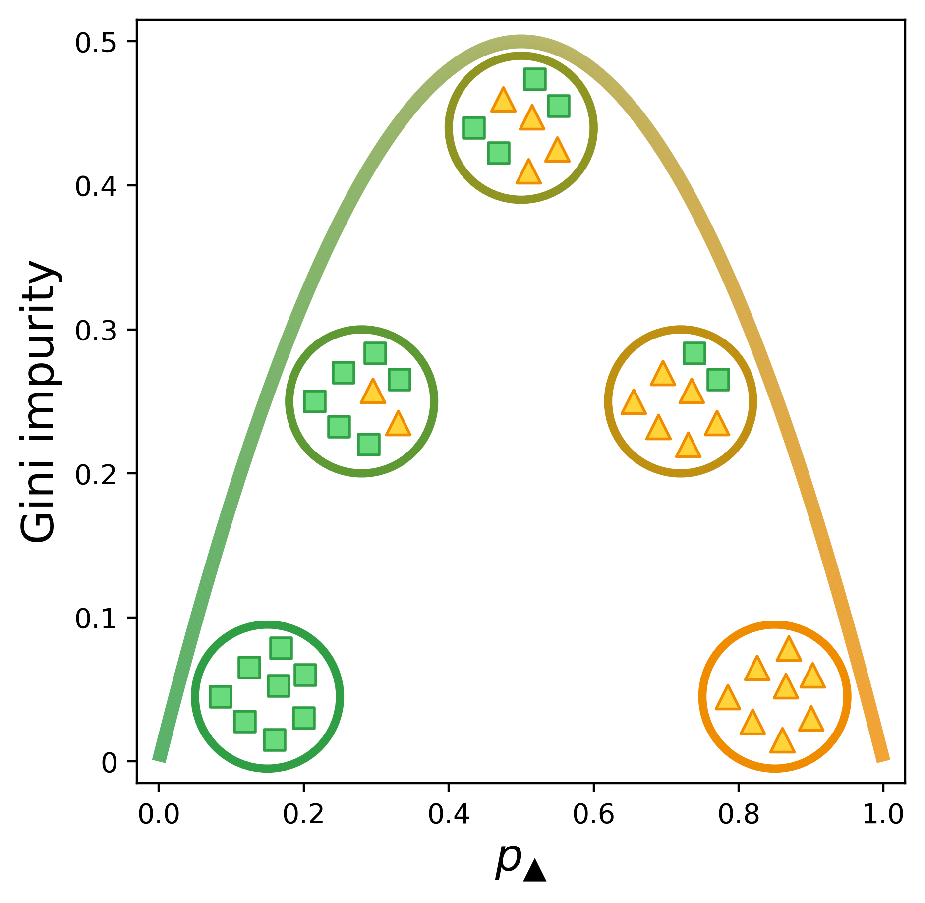
\[G = 1 - \sum_{k=1}^{m}{p_k}^2\]Here, $p_k$ is the probability of a randomly-drawn sample belonging to class $k$ among our $m$ classes. For our squares and triangles, since we only have two classes and the probabilities must sum to 1, we can just define the whole equation in terms of $p_k$.
\[G = 1 - {p_k}^2 - (1-p_k)^2\]Below is a visual representation of the Gini impurity as a function of $p_\checkmark$, the probability of randomly selecting a positive label from the set.[1] (We’ve just replaced $p_k$ with $p_\checkmark$ to indicate that the checkmarks are the positive class.) The lowest impurity is when the elements in the set are either all not checkmarks (i.e., x’s) or all checkmarks. The impurity peaks when we have equal numbers of x’s and checkmarks.
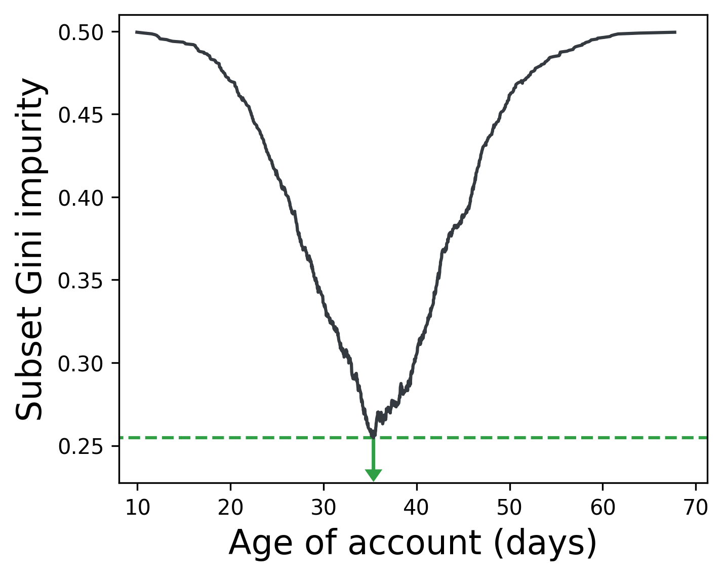
When identifying rules to partition our classes, then, we can simply select a split such that we minimize the weighted Gini impurity of the subsets. (Each subset has its own impurity, so we take the average weighted by the number of samples in each subset.) For a given feature, we can split the data on all possible values of that feature, record the weighted Gini impurity of the subsets, and then select the feature value that resulted in the lowest impurity.
Below, splitting the feature Age of account on 35 days best separates users who buy a product from those who don’t (in an imaginary dataset).
We can repeat this process for all features and select the feature whose optimal split resulted in the lowest impurity. Below, we see that the optimal split for Session length results in a lower Gini impurity than the best splits for Age of account and Is frequent shopper. Is frequent shopper is a binary feature, so there’s only one value to split with.
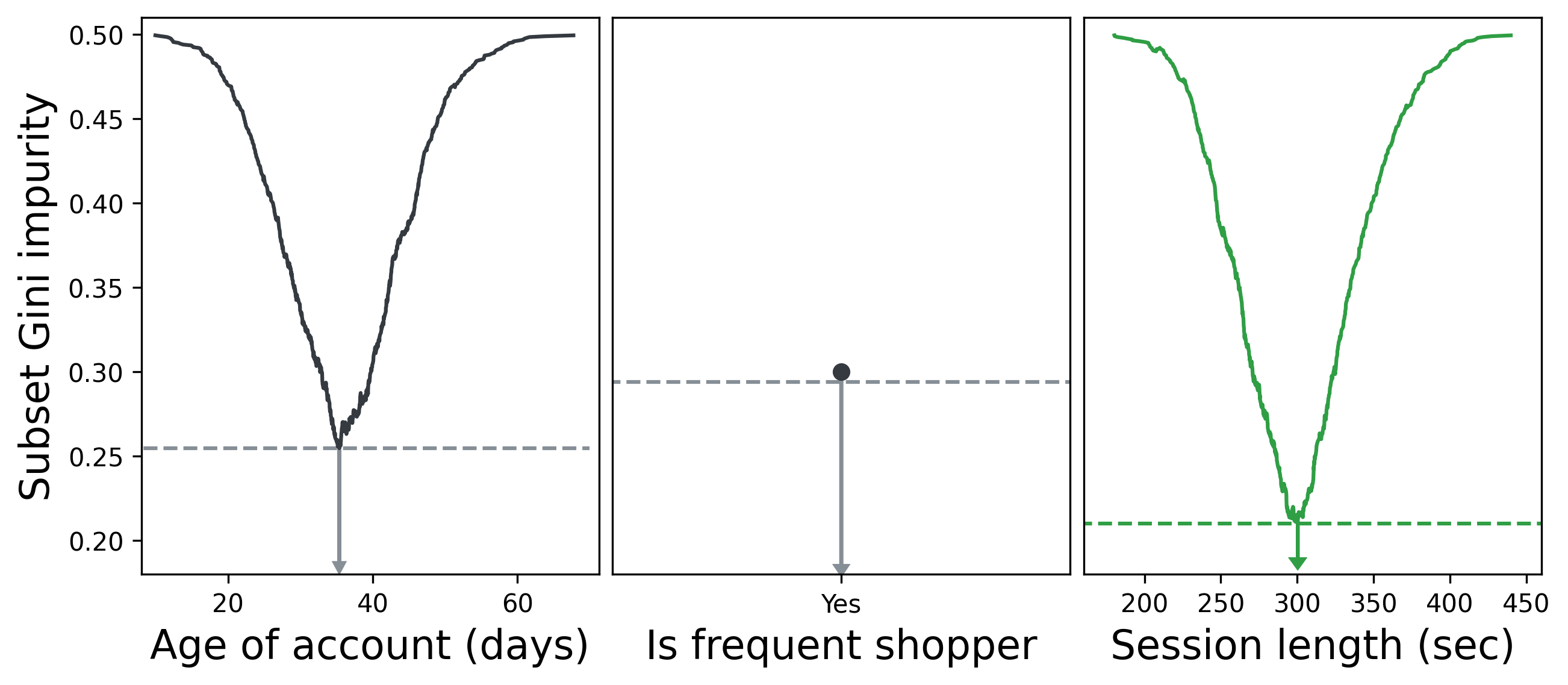
Splitting on Session length > 5 min therefore becomes the first fork in our decision tree. We then repeat our process of iterating through features and values and choosing the feature that best partitions the data for each subset, then their subsets, and so on until we either have perfectly partitioned data or our tree reaches a maximum allowed depth. (More on that in the next section.)
Below is the tree we saw earlier but with the training data displayed in each node. Notice how the positive and negative classes become progressively separated as we move down the tree. Once we reach the bottom of the tree, the leaf nodes output the majority class – the only class, in our case – in their data subset.
Random forests
The decision tree above partitions the data until the subsets contain only labels of one class (i.e., Gini impurity = 0). While this maximizes our model’s ability to explain its training data, we risk overfitting our model to our data. Think of it like the model memorizing every feature-label combination rather than learning the underlying patterns. An overfit model struggles to generalize to new data, which is usually our goal with modeling in the first place.
There are a few ways to combat overfitting. One option is to limit the depth of the tree. If we limited the above tree to only two levels, for example, we would end the left branch at the Is frequent shopper split.
The leaf nodes on the left branch now have mixed labels in their subsets. Allowing for this “impurity” might seem suboptimal, but it’s a strong defense against noisy features: if Time idle and Age of account had predictive power in our training data just due to chance, a model that excluded those features would be better at generalizing to new data.
Limiting tree depth works well, but we can pair it with an even stronger strategy: ensemble learning. In machine learning – and in animal collectives – aggregating a set of predictions often achieves higher accuracy than any individual prediction. Errors in individual models cancel out, allowing a clearer look at the underlying patterns in the data being modeled.
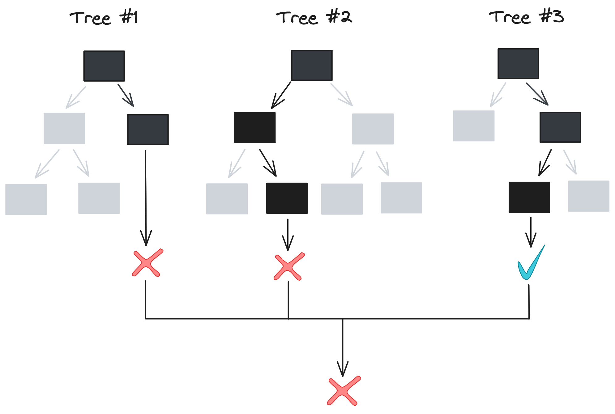
This sounds great, but there needs to be variation in model predictions for an ensemble to be useful. The algorithm we described in the last section – splitting on all values of all features to get the lowest Gini impurity – is deterministic. For a given dataset, our algorithm always outputs the same decision tree[2], so training 10 or 100 trees as an ensemble wouldn’t actually accomplish anything. So how is a forest any better than an individual tree?
This is where randomness comes in. Both the way our data is split and the data itself varies between trees in a random forest, allowing for variation in model predictions and greater protection against overfitting.
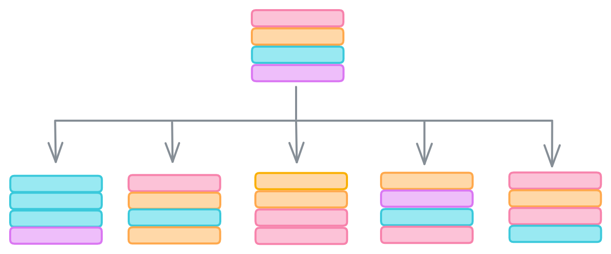
Let’s start with the data. We can protect against outliers hijacking our model with meaningless correlations by bootstrapping our data, or sampling with replacement. The idea is that outliers are rare, so they’re less likely to be randomly selected than samples reflecting genuine relationships between features and labels. Bootstrapping lets us give each decision tree in our forest a slightly different dataset that should still contain the same general trends.
The second way is that random forests randomly select only a subset of the features when evaluating how to split the data. scikit-learn’s RandomForestClassifier, for example, only considers the square root of the number of features when searching for the thresholds that minimize Gini impurity.
These methods might seem strange – why wouldn’t we use all our features, and why would we purposely duplicate and drop rows in our data? And indeed, each individual tree we produce this way often has significantly worse predictive power than a normal decision tree. But when we aggregate dozens of these Swiss-cheese trees, a surprising result emerges: a forest that is collectively more accurate than our original decision trees.
Implementation
Let’s now implement a random forest in Python to see for ourselves. We’ll start with the nodes of a tree, followed by a decision tree and finally a random forest.
Node
Let’s start with a class that will serve as a node in our decision tree. The class will have the following attributes used for training:
- A subset of data (or entire dataset for the root node)
- The proportion of positive labels and Gini impurity of this subset
- Pointers to left and right child nodes, set to
Noneif the node is a leaf
The class will also have the following attributes for classifying new data:
- A feature name and threshold, used to point the input towards the left or right child node (if the node is not a leaf)
- Which label to return (if the node is a leaf)
We can construct a Node class that meets these criteria with the below code. While the source code in GitHub has more thorough docstrings and input validation, I’ll share a slimmed down version here for readability. Note that we’ll call this file node.py and reference it in later files.
| Python |
1
2
3
4
5
6
7
8
9
10
11
12
13
14
15
16
17
18
19
20
21
22
23
24
25
26
27
28
29
30
31
32
33
34
35
36
37
38
39
40
import numpy as np
import pandas as pd
from typing_extensions import Self

class Node:
    """
    Node in a decision tree.
    """
    def __init__(
        self,
        df: pd.DataFrame,
        target_col: str
    ) -> None:
        # For training
        self.df = df
        self.target_col = target_col
        self.pk = self._set_pk()
        self.gini = self._set_gini()

        # For training/inference
        self.left = None
        self.right = None

        # For inference
        self.feature = None
        self.threshold = None

    def _set_pk(self) -> float:
        """
        Sets pk, the prop samples that are the positive class.
        Assumes samples are an array of ints, where 1 is the positive
        class and 0 is the negative class.
        """
        return np.mean(self.df[self.target_col].values)

    def _set_gini(self) -> float:
        """
        Sets the Gini impurity.
        """
        return 1 - self.pk**2 - (1 - self.pk)**2
So far the code is fairly lightweight. We instantiate the node by specifying a dataframe (df) and the column containing labels (target_col). We create empty attributes for the left and right child nodes (self.left, self.right) and the feature and threshold values used for inference. Finally, we calculate $p_k$ (the proportion of 1’s in target column) and the Gini impurity with the _set_pk and _set_gini methods, respectively.
Now let’s add the logic for iterating through the values of a feature and identifying the threshold that minimizes the Gini impurity in the child nodes. The function split_on_feature runs the helper function _process_split on each unique value in a feature. If any values are left after removing nulls (for leaf nodes, the list will be empty), we return the Gini impurity, feature threshold, and left and right child nodes for the split that resulted in the lowest impurity.
| Python |
1
2
3
4
5
6
7
8
9
10
11
12
13
14
15
16
17
18
19
20
21
class Node:
    ...
    def split_on_feature(
        self,
        feature: str
    ) -> tuple[float, int|float, Self, Self]:
        """
        Iterate through values of a feature and identify split that
        minimizes weighted Gini impurity in child nodes. Returns tuple
        of weighted Gini impurity, feature threshold, and left and
        right child nodes.
        """
        values = []

        for thresh in self.df[feature].unique():
            values.append(self._process_split(feature, thresh))

        values = [v for v in values if v[1] is not None]
        if values:
            return min(values, key=lambda x: x[0])
        return None, None, None, None
Here’s _process_split, which does the actual work. We split self.df on the feature threshold, end early if either child dataset is empty, create child nodes with the subsets, and finally calculate the weighted Gini impurity.
| Python |
1
2
3
4
5
6
7
8
9
10
11
12
13
14
15
16
17
18
19
20
21
22
23
24
25
26
27
28
29
class Node:
    ...
    def _process_split(
        self,
        feature: str,
        threshold: int|float
    ) -> tuple[float, int|float, Self|None, Self|None]:
        """
        Splits df on the feature threshold. Returns weighted Gini
        impurity, inputted threshold, and child nodes. If split
        results in empty subset, returns Gini impurity and None's.
        """
        df_lower = self.df[self.df[feature] <= threshold]
        df_upper = self.df[self.df[feature] > threshold]

        # If threshold doesn't split the data at all, end early
        if len(df_lower) == 0 or len(df_upper) == 0:
            return self.gini, None, None, None

        node_lower = Node(df_lower, self.target_col)
        node_upper = Node(df_upper, self.target_col)

        prop_lower = len(df_lower) / len(self.df)
        prop_upper = len(df_upper) / len(self.df)

        weighted_gini = node_lower.gini * prop_lower \
          + node_upper.gini * prop_upper

        return weighted_gini, threshold, node_lower, node_upper
Let’s quickly test it out. Below, we instantiate a node and have it find the optimal split for the data. split_on_feature returns the weighted Gini impurity of 0.0 in the child nodes because we can perfectly partition the labels at a value of 2 (the second returned value). The third and fourth values are the left and right child nodes from the partitioning.
| Python |
1
2
3
4
5
6
7
8
9
10
11
12
import pandas as pd

df = pd.DataFrame({'feature': [1, 2, 3], 'label': [0, 0, 1]})
node = Node(df, 'label')

print(f"pk: {round(node.pk, 2)}, gini: {round(node.gini, 2)}")
# pk: 0.33, gini: 0.44

print(node.split_on_feature('feature'))
# (0.0, 2,
# <__main__.Node object at 0x137c279d0>,
# <__main__.Node object at 0x137c24160>)
Decision tree
The next step is to arrange nodes in a tree to best partition training data and most accurately classify new data. Let’s start with the basic structure, then the ability to train the classifier (i.e., build the tree) and generate predictions. We store our decision_tree.py file in the same directory as node.py and import Node from the file.
Our DecisionTree class begins with the root node, which is a Node we instantiate with df and target_col. feature_select controls the proportion of features we use when training the trees of a random forest; we’ll default to 100% of features for the base decision tree class. max_depth specifies the maximum depth our tree can grow, which helps prevent overfitting.
| Python |
1
2
3
4
5
6
7
8
9
10
11
12
13
14
15
16
17
18
19
20
21
import numpy as np
import pandas as pd

from .node import Node

class DecisionTree:
    """
    Decision tree classifier, constructed with Nodes
    """
    def __init__(
        self,
        df: pd.DataFrame,
        target_col: str,
        feature_select: float = 1.0,
        max_depth: int = 4
    ) -> None:
        self.root = Node(df, target_col)
        self.features = list(df)
        self.features.remove(target_col)
        self.feature_select = feature_select
        self.max_depth = max_depth
Now let’s write the logic to build the tree. Proving that all that Leetcode I studied is useful outside of just coding interviews, we use a stack to perform a depth-first traversal, iteratively calling _process_node on each node and appending its children to the stack. We also keep an eye on our current depth to ensure we don’t exceed self.max_depth. Once we’ve processed all nodes, we return our DecisionTree instance.
| Python |
1
2
3
4
5
6
7
8
9
10
11
12
13
14
15
16
17
18
19
20
21
class DecisionTree:
    ...
    def build_tree(self) -> None:
        """
        Builds tree using depth-first traversal
        """
        stack = [(self.root, 0)]

        while stack:
            current_node, depth = stack.pop()

            if depth <= self.max_depth:
                left, right = self._process_node(current_node)

                if left and right:
                    current_node.left = left
                    current_node.right = right
                    stack.append((right, depth+1))
                    stack.append((left, depth+1))

        return self
What actually happens in _process_node? We start by randomly selecting a subset of features (or just all of them if self.feature_select is 1.0), followed by iterating through those features and calling the node’s split_on_feature method to find that feature’s optimal split. We then find the feature whose split resulted in the lowest Gini impurity in the child nodes and compare it to our current node’s impurity. If the best split resulted in a lower impurity, we return the child nodes; if not, we return None to indicate we should stop traversing.
| Python |
1
2
3
4
5
6
7
8
9
10
11
12
13
14
15
16
17
18
19
20
21
22
23
24
25
26
27
28
29
30
31
32
33
34
35
36
37
38
39
40
41
42
43
44
45
class DecisionTree:
    ...
    def _process_node(
        self,
        node: Node
    ) -> tuple[Node|None, Node|None]:
        """
        Iterates through features, identifies split that minimizes
        Gini impurity in child nodes, and identifies feature whose
        split minimizes Gini impurity the most. Then returns child
        nodes split on that feature.
        """
        # Randomly select features. No randomness if
        # self.feature_select = 1.0 (default).
        features = list(
            np.random.choice(
                self.features,
                int(self.feature_select*len(self.features)),
                replace=False
            )
        )

        # Get Gini impurity for best split for each column
        d = {}
        for col in features:
            feature_info = node.split_on_feature(col)
            if feature_info[0] is not None:
                d[col] = feature_info

        # Select best column to split on
        min_gini = np.inf
        best_feature = None
        for col, tup in d.items():
            if tup[0] < min_gini:
                min_gini = tup[0]
                best_feature = col

        # Only update if the best split reduces Gini impurity
        if min_gini < node.gini:
            # Update node
            node.feature = best_feature
            node.threshold = d[col][1]
            return d[col][2:]

        return None, None
The above code allows us to build a tree. Now let’s write the code for generating predictions.
Our classify function is just a wrapper around the helper _classify and lets us generate predictions on a dataframe of feature vectors (rather than just one at a time). The real work is done in _classify, which recursively moves to the left or right child node depending on how the feature vector compares to the node’s threshold. A leaf node has None for its feature and threshold attributes, so we then return a label of 1 if the node’s $p_k$ is greater than 0.5, else 0.
| Python |
1
2
3
4
5
6
7
8
9
10
11
12
13
14
15
16
17
18
19
20
21
22
23
24
25
class DecisionTree:
    ...
    def classify(self, feature_df: pd.DataFrame) -> list[int]:
        """
        Given a dataframe where each row is a feature vector, traverses
        the tree to generate a predicted label.
        """
        return [
          self._classify(self.root, f) for i, f in feature_df.iterrows()
        ]

    def _classify(self, node: Node, features: pd.Series) -> int:
        """
        Given a vector of features, traverse the node's children until
        a leaf is reached, then return the most frequent class in the
        node. If there are an equal number of positive and negative
        labels, predicts the negative class.
        """
        # Child node
        if node.feature is None or node.threshold is None:
            return int(node.pk > 0.5)

        if features[node.feature] < node.threshold:
            return self._classify(node.left, features)
        return self._classify(node.right, features)
Random Forest
We have everything we need for a decision tree classifier! The hardest work – by far – is behind us. Extending our classifier to a random forest just requires generating multiple trees on bootstrapped data, since we’ve already implemented randomized feature selection in _process_node.
So let’s create a random_forest.py file that contains a RandomForest class. As always, we instantiate the class with a dataframe (df) and target column, and like the DecisionTree class we have a feature_select and max_depth parameter. Instantiation now also takes an n_trees parameter.
| Python |
1
2
3
4
5
6
7
8
9
10
11
12
13
14
15
16
17
18
19
20
21
22
import pandas as pd

from .decision_tree import DecisionTree

class RandomForest:
    """
    Forest of decision trees.
    """
    def __init__(
        self,
        df: pd.DataFrame,
        target_col: str,
        n_trees: int = 100,
        feature_select: float = 0.5,
        max_depth: int = 4
    ) -> None:
        self.df = df
        self.target_col = target_col
        self.n_trees = n_trees
        self.feature_select = feature_select
        self.max_depth = max_depth
        self.forest = []
Training is straightforward: we create n_trees bootstrapped dataframes, instantiate a DecisionTree for each one, then call .build_tree to train each decision tree.
| Python |
1
2
3
4
5
6
7
8
9
10
11
12
13
14
15
16
17
18
19
20
21
22
23
24
class RandomForest:
    ...
    def train(self) -> None:
        """
        Fit the forest to self.df
        """
        bootstrap_dfs = [self._bootstrap() for _ in range(self.n_trees)]
        self.forest = [
            DecisionTree(
              bdf,
              self.target_col,
              self.feature_select,
              self.max_depth
            )
            for bdf in bootstrap_dfs
        ]
        self.forest = [tree.build_tree() for tree in self.forest]
        return None

    def _bootstrap(self) -> pd.DataFrame:
        """
        Sample rows from self.df with replacement
        """
        return self.df.sample(len(self.df), replace=True)
Classification is also simple: we have each tree in the forest classify the inputted feature_df, then return the most common predicted label for each row. I found that the easiest way to do this was to cast the preds list to a dataframe and then take the mode.
1
2
3
4
5
6
7
8
9
10
11
12
13
class RandomForest
    ...
    def classify(self, feature_df: pd.DataFrame) -> int:
        """
        Classify inputted feature vectors. Each tree in the forest
        generates a predicted label and the most common label for
        each feature vector is returned.
        """
        preds = pd.DataFrame(
          [tree.classify(feature_df) for tree in self.forest]
        )
        # Return most common predicted label
        return list(preds.mode().iloc[0])
And… that’s it! If we run the script run.py, we can compare the accuracies of our DecisionTree classifier, the average tree in a RandomForest, the full RandomForest, and scikit-learn’s RandomForestClassifier for good measure. The results will vary by dataset, number of trees per forest, etc., but we can see that our lone decision tree has higher accuracy than the average tree in the forest, and that the full random forest is substantially stronger than individual trees. Unsurprisingly, scikit-learn has the highest accuracy… but we didn’t do too badly!
| bash |
1
2
3
4
5
Accuracy
 * Single decision tree:   0.61
 * Avg random forest tree: 0.595
 * Full random forest:     0.81
 * Scikit-learn forest:    0.89
Conclusions
In this post, we covered one of the most popular and powerful algorithms in machine learning: the random forest. We started with the theory, explaining how decision trees use metrics such as Gini impurity to identify the value of a feature that best splits a dataset. We then showed how we can build a tree by iteratively identifying the feature whose optimal split most reduces Gini impurity until the classes are either perfectly separated or we reach a maximum accepted depth. We explained how a random forest is constructed with dozens of decision trees, random feature selection, and bootstrapped datasets. Finally, we wrote some code to test the theory.
If you’re hungry for more, there are plenty of mini projects to try. You could visualize how the same feature can be used multiple times in a tree if it has a highly non-linear relationship with the target variable. We didn’t cover regression in this post, but it wouldn’t take much effort to modify our code to handle a continuous target. It’d be interesting to see how the predictive power of the vanilla DecisionTree, the average random forest tree, and the full forest diverge as a function of the amount of data and number of columns. Finally, if anyone wants to parallelize how RandomForest trains trees, feel free to submit a PR. 😜
Thanks for reading!
Matt
Footnotes
1. Decision tree training
This figure was a serious labor of love. Figuring out how to get the curve (and circles) to transition from one color to another was tricky, but surprisingly the hardest part was dealing with the spacing of the x’s and checkmarks to keep them cleanly within the circles but not too bunched up. I changed the icons and colors of this figure so many times that I ended up writing a script to generate it.
Here’s a version of the figure I had for a while before I thought I needed a clearer visual distinction from the toy example (partitioning shapes) and the main example in the post (e-commerce).
2. Random forests
You can see for yourself how sklearn outputs identical decision trees for a given dataset with the below code. Note that we need to specify the same random_state.
| Python |
1
2
3
4
5
6
7
8
9
10
11
12
13
14
15
16
17
18
19
20
21
22
23
24
25
import numpy as np
import pandas as pd
from sklearn.tree import DecisionTreeClassifier

# Params
random_state = 42

# Generate data
df = pd.DataFrame(
    {
        'feature_1': np.random.normal(0, 1, 100),
        'feature_2': np.random.normal(1, 1, 100),
        'label': np.random.choice([0, 1], 100)
    }
)

mod1 = DecisionTreeClassifier(random_state=random_state)
mod1.fit(df[['feature_1', 'feature_2']], df['label'])

mod2 = DecisionTreeClassifier(random_state=42)
mod2.fit(df[['feature_1', 'feature_2']], df['label'])

comparison = (mod1.tree_.value == mod2.tree_.value)
print(comparison.all())
# True