
A hands-on demo of analyzing big data with Spark
#pythonWritten by Matt Sosna on June 16, 2021
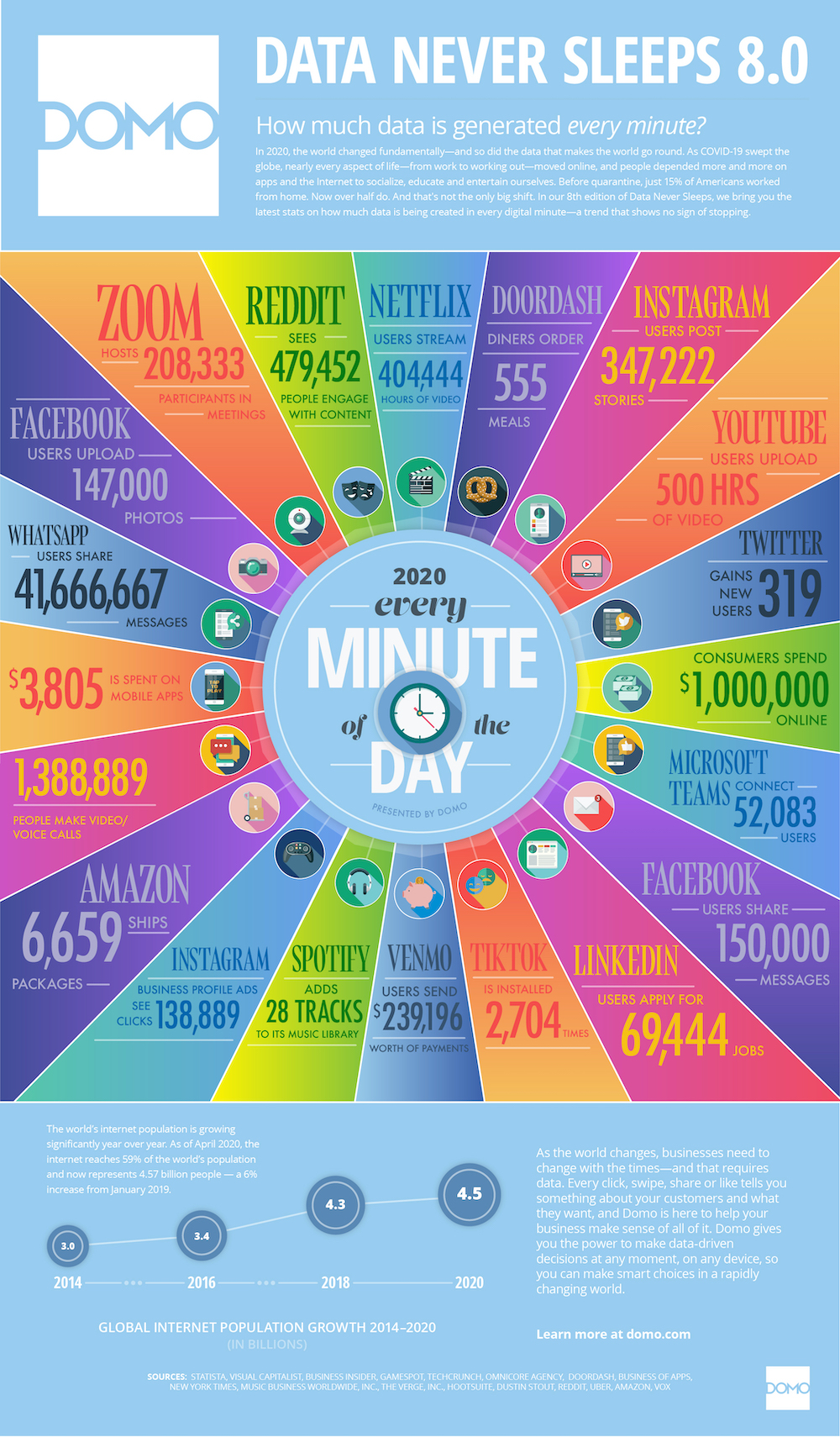
Cloud services firm Domo estimates that for every minute in 2020, WhatsApp users sent 41.7 million messages, Netflix streamed 404,000 hours of video, $240,000 changed hands on Venmo, and 69,000 people applied for jobs on LinkedIn. In that firehose of data are patterns those companies use to understand the present, predict the future, and ultimately stay alive in a hyper-competitive market.
But how is it possible to extract insights from datasets so large they freeze your laptop when you try to load them into pandas? When a dataset has more rows than dollars the median U.S. household will earn in 50 years[1], we could head to BestBuy.com, sort their computers by “most expensive,” and shell out some cash for a fancy machine.
Or we could try Apache Spark.
By the end of this post, you’ll understand why you don’t need expensive hardware to analyze massive datasets $-$ because you’ll have already done it. We’ll cover what Spark is before counting the frequency of each letter in a novel, calculating $\pi$ by hand, and processing a dataframe with 50 million rows.
Table of contents
- The analytics framework for big data
- Counting letter frequencies in a novel
- Calculating $\pi$
- Spark dataframes and machine learning
The analytics framework for big data
Spark is a framework for processing massive amounts of data. It works by partitioning your data into subsets, distributing the subsets to worker nodes (whether they’re logical CPU cores on your laptop[2] or entire machines in a cluster), and then coordinating the workers to analyze the data. In essence, Spark is a “divide and conquer” strategy.
A simple analogy can help visualize the value of this approach. Let’s say we want to count the number of books in a library. The “expensive computer” approach would be to teach someone to count books as fast as possible, training them for years to accurately count while sprinting. While fun to watch, this approach isn’t that useful $-$ even Olympic sprinters can only run so fast, and you’re out of luck if your book-counter gets injured or decides to change professions!
The Spark approach, meanwhile, would be to get 100 random people, assign each one a section of the library, have them count the books in their section, and then add their answers together. This approach is more scalable, fault-tolerant, and cheaper… and probably still fun to watch.
Spark’s main data type is the resilient distributed dataset (RDD). An RDD is an abstraction of data distributed in many places, like how the entity “Walmart” is an abstraction of millions of people around the world. Working with RDDs feels like manipulating a simple array in memory, even though the underlying data may be spread across multiple machines.
Getting started
Spark is mainly written in Scala but can be used from Java, Python, R, and SQL. We’ll use PySpark, the Python interface for Spark. To install PySpark, type pip install pyspark in the Terminal. You might also need to install or update Java. You’ll know everything is set up when you can type pyspark in the Terminal and see something like this.
| bash |
1
2
3
4
5
6
7
8
9
10
11
Welcome to
      ____              __
     / __/__  ___ _____/ /__
    _\ \/ _ \/ _ `/ __/  '_/
   /__ / .__/\_,_/_/ /_/\_\   version 3.1.2
      /_/

Using Python version 3.7.4 (default, Sep  7 2019 18:27:02)
Spark context Web UI available at http://matts-mbp:4041
Spark context available as 'sc' (master = local[*], app id = local-123).
SparkSession available as 'spark'.
The rest of the code in this post can be run in the Spark terminal as above, or in a separate Python or Jupyter instance. I’ll run the rest of the code in Jupyter so we can have access the incredibly handy %%timeit IPython magic command for measuring the speed of code blocks.
Below is a tiny PySpark demo. We start by manually defining the SparkSession to start a connection to Spark. (If you’re in the PySpark Terminal, this is already done for you.) We then create an RDD of an array, visualize the first two numbers, and print out the maximum. With .getNumPartitions, we see that Spark allocated our array to the eight logical cores on my machine.
| Python |
1
2
3
4
5
6
7
8
9
10
11
12
13
from pyspark.sql import SparkSession

# Start Spark connection
spark = SparkSession.builder.getOrCreate()

# Allocate the numbers 0-999 to an RDD
numbers = range(1000)
rdd = spark.sparkContext.parallelize(numbers)

# Visualize RDD
print(rdd.take(2))  # [0, 1]
print(rdd.max())    # 999
print(rdd.getNumPartitions())  # 8
With this basic primer, we’re ready to start leveraging Spark to process large datasets. Since you probably don’t have any terabyte- or petabyte-size datasets lying around to analyze, we’ll need to get a little creative. Let’s start with a novel.
Counting letter frequencies in a novel
Project Gutenberg is an online repository of books in the public domain, so we can pull a book from there to analyze. Let’s do Leo Tolstoy’s War and Peace $-$ I’ve always wanted to read it, or at least know how frequently each letter in the alphabet appears! [3]
Below, we get the HTML from the novel’s webpage with the Beautiful Soup Python library, tidy up the paragraphs, and then append them to a list. We then remove the first 383 paragraphs that are just the table of contents! We’re left with 11,186 paragraphs ranging from 4 characters to 4381. (The string kind of characters, but with War and Peace, maybe novel characters too.)
| Python |
1
2
3
4
5
6
7
8
9
10
11
12
13
14
15
16
17
18
19
20
21
22
23
24
25
26
27
28
29
30
31
32
33
34
35
36
37
38
39
40
41
42
43
44
45
46
import requests
import pandas as pd
from bs4 import BeautifulSoup

# Pull book
book_url = "https://www.gutenberg.org/files/2600/2600-h/2600-h.htm"
response = requests.get(book_url)
soup = BeautifulSoup(response.text, 'html')

# Create list to store clean paragraphs
pars = []

# Set minimum str length for paragraphs
MIN_PAR_LEN = 2

# Iterate through paragraphs
for par in soup.findAll('p'):

    # Remove newlines and returns
    par_clean = ''.join(par.text.split('\n'))
    par_clean = ''.join(par_clean.split('\r'))

    if par_clean == '':
        continue

    # Remove extra spaces
    par_clean = par_clean.split('  ')
    par_clean = ' '.join([p for p in par_clean if p != ''])

    # Add cleaned paragraph to list
    if len(par_clean) > MIN_PAR_LEN:
        pars.append(par_clean)

# Remove table of contents
pars = pars[383:]

# Visualize paragraph lengths
pd.Series([len(par) for par in pars]).describe().astype(int)
# count    11186
# mean       284
# std        337
# min          4
# 25%         84
# 50%        170
# 75%        347
# max       4381
Despite War and Peace being a massive novel, we see that pandas can still process high-level metrics without a problem $-$ line 38 runs nearly instantly on my laptop.
But we’ll start to notice a substantial performance improvement with Spark when we start asking tougher questions, like the frequency of each letter throughout the book. This is because the paragraphs can be processed independently from one another; Spark will process paragraphs several at a time, whereas Python and pandas will process them one by one.
As before, we start our Spark session and create an RDD of our paragraphs. We also load Counter, a built-in Python class optimized for counting, and reduce, which we’ll use to demo the base Python approach later.
| Python |
1
2
3
4
5
6
7
8
9
from functools import reduce
from collections import Counter
from pyspark.sql import SparkSession

# Create Spark session
spark = SparkSession.builder.getOrCreate()

# Partition novel into RDD
rdd = spark.sparkContext.parallelize(pars)
We then map the Counter command to each paragraph with rdd.map(Counter). Note how nothing happens unless we add .take(2) to output the first two results $-$ Spark does lazy evaluation, a method for optimizing chains of queries until a result actually needs to be returned.
| Python |
1
2
3
4
5
6
7
8
9
10
11
12
13
14
15
16
17
18
19
20
# Nothing happens
rdd.map(Counter)
# PythonRDD[12] at RDD at PythonRDD.scala:53

# We force the execution by asking to display 1st two results
rdd.map(Counter).take(2)
# [Counter({'“': 1,
#           'W': 1,
#           'e': 40,
#           ...
#           '!': 1,
#           '?': 1,
#           '”': 1}),
#  Counter({'I': 1,
#           't': 19,
#           ' ': 79,
#           ...
#           'K': 1,
#           ';': 1,
#           'b': 3})]
rdd.map(Counter) gives us a new RDD with the letter frequencies for each paragraph, but we actually want the letter frequencies of the entire book. Fortunately, we can do this by simply adding the Counter objects together.
We perform this reduction from a multi-element RDD to a single output with the .reduce method, passing in an anonymous addition function to specify how to collapse the RDD.[4] The result is a Counter object. We then finish our analysis by using its .most_common method to print out the ten most common characters.
| Python |
1
2
3
4
5
6
7
8
9
10
11
rdd.map(Counter).reduce(lambda x, y: x + y).most_common(10)
# [(' ', 554621),
#  ('e', 308958),
#  ('t', 217658),
#  ('a', 194793),
#  ('o', 186623),
#  ('n', 179202),
#  ('i', 162925),
#  ('h', 162216),
#  ('s', 158811),
#  ('r', 143914)]
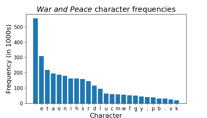
And the winner is… space! Here’s those same frequencies, but in a nice barplot.
Was using Spark worth it? Let’s end this section by timing how long it takes our task to run in Spark versus base Python. We can use the %%timeit IPython magic command in separate Jupyter notebook cells to see how our methods compare.
In Spark:
| Python |
1
2
3
%%timeit
rdd.map(Counter).reduce(lambda x, y: x + y).most_common(5)
# 272 ms ± 18.6 ms per loop (mean ± std. dev. of 7 runs, 1 loop each)
And in base Python:
| Python |
1
2
3
%%timeit
reduce(lambda x, y: x + y, (Counter(val) for val in pars)).most_common(5)
# 806 ms ± 9.37 ms per loop (mean ± std. dev. of 7 runs, 1 loop each)
With Spark, we’re about 67.7% faster than using base Python. Sweet! Now I need to decide what to do with that extra half second of free time.
Calculating $\pi$
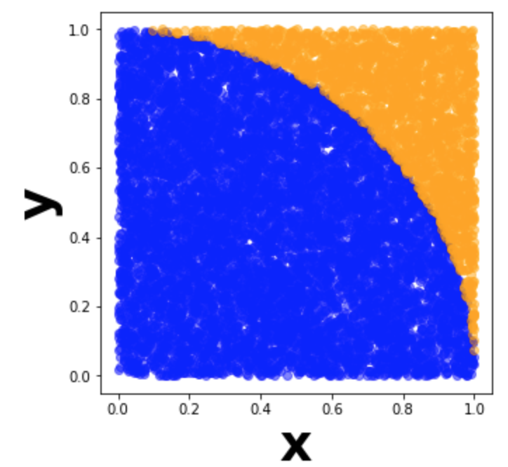
There are many great tutorials on how to calculate pi using random numbers. The brief summary is that we generate random x-y coordinates between (0,0) and (1,1), then calculate the proportion of those points that fall within a circle with radius 1. We can then solve for $\pi$ by multiplying this proportion by 4. In the visualization of 10,000 points below, we would divide the number of blue points by the total number of points to get $\frac{\pi}{4}$.
The more points we generate, the more accurate our estimate gets for $\pi$. This is an ideal use case for Spark, since the generated points are all independent. Rather than analyze pre-existing data, we can use our worker nodes to each generate thousands of points and calculate the proportion of those points that land inside the circle. We can then take the mean of our proportions for our final estimate of $\pi$.
Here’s the function we’ll have each worker run. I tried striking a balance between 1) generating one point each time (low memory but slow), versus 2) generating all samples at once and then calculating the proportion (efficient but can hit memory limits). A decent solution I found is to break n_points into several chunks, calculate the proportion of points within the circle for each chunk, and then get the mean of proportions at the end.
| Python |
1
2
3
4
5
6
7
8
9
10
11
12
13
14
15
16
17
18
import numpy as np

def calculate_pi(n_points, n_chunks=11):
    """
    Generate n_points coordinates between [0, 1), [0, 1) and count
    the proportion that fall within a unit circle. n_points/n_chunks
    points generated at a time.
    """
    means = []

    for _ in np.linspace(0, n_points, n_chunks):

        x = np.random.rand(int(n_points/n_chunks))
        y = np.random.rand(int(n_points/n_chunks))

        means.append(np.mean(np.sqrt(x**2 + y**2) < 1))

    return np.mean(means) * 4
Now let’s create an RDD and map calculate_pi to each element, then take the mean of each element’s estimate of $\pi$.
| Python |
1
2
3
4
5
6
7
8
9
10
from pyspark.sql import SparkSession
spark = SparkSession.builder.getOrCreate()

n_estimators = 100
n_samples = 1000000

rdd = spark.sparkContext.parallelize(range(n_estimators))

rdd.map(lambda x: calculate_pi(n_samples)).mean()
# 3.141782
Our estimate of pi isn’t too bad! Using %%timeit again, we see that on my machine, base Python takes about 3.67 s, while Spark takes 0.95 s, a 74% improvement. Nice!
Spark dataframes and machine learning
Let’s do one more example, this time using a nice abstraction Spark provides on top of RDDs. In a syntax similar to pandas, we can use Spark dataframes to perform operations on data that’s too large to fit into a pandas df. We can then train machine learning models with our dataframe.
Spark dataframes
You probably don’t have a dataframe with a few million rows laying around, so we’ll need to generate one. Since by definition we’re trying to create a dataset too large to fit into pandas, we’ll need to generate the dataframe in pieces, iteratively saving CSVs to later ingest with PySpark.
Let’s do 50 million rows, just for fun. We’ll generate 50 CSVs, each with 1,000,000 rows. Our data will consist of exam scores for four students, and the number of hours they spent studying vs. dancing the previous day. These are some students dedicated to big data $-$ they’ll be taking about 12.5 million exams each!
| Python |
1
2
3
4
5
6
7
8
9
10
11
12
13
14
15
16
17
18
19
20
21
22
23
24
25
26
27
28
29
30
31
32
33
34
35
36
37
import os
import numpy as np
import pandas as pd

# Create dataset folder to store CSVs
folder = "datasets"

if folder not in os.listdir():
    os.mkdir(folder)

# Define students and number of rows per CSV
students = ['Abby', 'Brad', 'Caroline', 'Dmitry']
n = 1000000

for i in range(1, 51):

    # Generate vector of random names
    names = np.random.choice(students, n)

    # Generate features with varying influence on exam score
    study = np.linspace(0, 8, n) + np.random.normal(0, 0.5, n)
    dance = np.linspace(0, 8, n) + np.random.normal(0, 10, n)

    # Generate scores
    score = np.linspace(0, 100, n) + np.random.normal(0, 0.5, n)

    # Group data together into df
    df_iter = pd.DataFrame({'name': names,
                            'study': study,
                            'dance': dance,
                            'score': score})

    df_iter.to_csv(f'{folder}/big_df_{i}.csv', index=False)

    # Log our progress
    if i % 5 == 0:
        print(f"{round(100*i/50)}% complete")
We’ll now create a Spark dataframe from the CSVs, visualize the schema, and print out the number of rows. But we’ll first need to add a configuration option when we define our Spark session $-$ for the following code blocks to run, I needed to double the driver memory to avoid crashing Spark! We’ll do this with the .config('spark.driver.memory', '2g') line.
| Python |
1
2
3
4
5
6
7
8
9
10
11
12
13
14
15
16
17
18
19
20
21
22
23
from pyspark.sql import SparkSession

# Define session and increase driver memory
spark = SparkSession.builder\
            .config('spark.driver.memory', '2g')\
            .getOrCreate()

# Create a Spark df from the CSVs
rdd_df = spark.read.format('csv')\
            .option('header', 'true')\
            .option('inferSchema', 'true')\
            .load(f'{folder}/big_df*')

rdd_df.printSchema()
# root
#  |-- name: string (nullable = true)
#  |-- study: double (nullable = true)
#  |-- sleep: double (nullable = true)
#  |-- dance: double (nullable = true)
#  |-- score: double (nullable = true)

rdd_df.count()
# 50000000
Let’s now analyze our data. We’ll start by counting the number of rows for each person.
| Python |
1
2
3
4
5
6
7
8
9
rdd_df.groupBy('name').count().orderBy('name').show()
# +--------+--------+
# |    name|   count|
# +--------+--------+
# |    Abby|12502617|
# |    Brad|12505754|
# |Caroline|12497831|
# |  Dmitry|12493798|
# +--------+--------+
12.5 million exams each… incredible. Now let’s find the average of the hours studied, hours danced, and exam scores by person.
| Python |
1
2
3
4
5
6
7
8
9
rdd_df.groupBy('name').mean().orderBy('name').show()
# +--------+------------------+------------------+------------------+
# |    name|        avg(study)|        avg(dance)|        avg(score)|
# +--------+------------------+------------------+------------------+
# |    Abby| 4.000719675263846| 4.003064539205431| 50.00863317710569|
# |    Brad| 4.000347945431657|3.9951049814089465|50.003555427979684|
# |Caroline|3.9990820375739693| 3.997358096942248| 49.99076907377133|
# |  Dmitry|3.9999589716292063|3.9977244162538814| 49.99676120966577|
# +--------+------------------+------------------+------------------+
Unsurprisingly, there’s no variation between people since we didn’t specify any when generating the data. The means are also right in the middle of the ranges specified on the data: 0-8 for hours, and 0-100 for scores.
To make those values nice and rounded, we’ll actually need to create a user-defined function (UDF). For a function we can apply to a groupby operation, we’ll load in pandas_udf and PandasUDFType. We also import DoubleType, which refers to the data type of the returned value from our function. After defining our function, we use spark.udf.register to make it available to our Spark environment.
| Python |
1
2
3
4
5
6
7
8
from pyspark.sql.types import DoubleType
from pyspark.sql.functions import pandas_udf, PandasUDFType

@pandas_udf(DoubleType(), functionType=PandasUDFType.GROUPED_AGG)
def round_mean(vals):
    return round(vals.mean(), 4)

spark.udf.register("round_mean", round_mean)
Now we can apply it to our dataframe. Note that since we’re using .agg, we’ll need to pass in a dictionary with the columns we want to apply our UDF to. Rather than type out {'study': 'round_mean', 'dance': 'round_mean', 'score': 'round_mean'}, I used a dictionary comprehension to be fancy. Though it’s probably the same number of keystrokes…
| Python |
1
2
3
4
5
6
7
8
9
10
11
func_dict = {col: 'round_mean' for col in rdd_df.columns[1:]}

rdd_df.groupBy('name').agg(func_dict).orderBy('name').show()
# +--------+-----------------+-----------------+-----------------+
# |    name|round_mean(score)|round_mean(study)|round_mean(dance)|
# +--------+-----------------+-----------------+-----------------+
# |    Abby|          50.0086|           4.0007|           4.0031|
# |    Brad|          50.0036|           4.0003|           3.9951|
# |Caroline|          49.9908|           3.9991|           3.9974|
# |  Dmitry|          49.9968|              4.0|           3.9977|
# +--------+-----------------+-----------------+-----------------+
Much cleaner! UDFs are a powerful tool for applying calculations to our data that don’t already come with PySpark.
Machine learning
Finally, let’s run a linear regression on our data. When training models, you’re probably used to having your feature vectors spread out across columns in a dataframe, one per feature. In sklearn, for example, we could just fit a model directly on the score column vs. the ['study', 'dance'] columns.
Spark, however, expects the entire feature vector for a row to reside in one column. We’ll therefore use VectorAssembler to turn our study and dance values into a new features column of 2-element vectors.
| Python |
1
2
3
4
5
6
7
8
9
10
11
12
13
14
from pyspark.ml.feature import VectorAssembler

# Create a reformatted df
assembler = VectorAssembler(inputCols=['study', 'dance'],
                            outputCol='features')
df_assembled = assembler.transform(rdd_df)
df_assembled.show(2)
# +------+--------+--------+--------+--------------------+
# |  name|   study|   dance|   score|            features|
# +------+--------+--------+--------+--------------------+
# |Dmitry|0.036...|-9.30...|-0.52...|[0.036..., -9.30...]|
# |  Abby|-0.63...|8.582...|-0.28...|[-0.63..., 8.582...]|
# +------+--------+--------+--------+--------------------+
# only showing top 2 rows
Now we actually fit our model. We split our data into training and test sets, then use the LinearRegression class to find the relationship between features and score. Finally, we visualize our coefficients and their p-values before calculating the RMSE on our test set.
| Python |
1
2
3
4
5
6
7
8
9
10
11
12
13
14
15
16
17
18
19
20
21
22
23
24
25
from pyspark.ml.regression import LinearRegression
from pyspark.ml.evaluation import RegressionEvaluator

# Split into train (70%) vs. test (30%) data
splits = df_assembled.randomSplit([0.7, 0.3])
df_train = splits[0]
df_test = splits[1]

# Define LinearRegression object
lr = LinearRegression(featuresCol='features', labelCol='score')

# Fit model and visualize coefficients
lr_model = lr.fit(df_train)
print(lr_model.intercept)       # 2.2327
print(lr_model.coefficients)    # [11.912, 0.0297]
print(lr_model.summary.pValues) # [0.0, 0.0, 0.0]

# Generate predictions to compare to actuals
lr_predictions = lr_model.transform(df_test)
lr_evaluator = RegressionEvaluator(predictionCol="prediction",
                                   labelCol="score",
                                   metricName="rmse")

# Evaluate RMSE on test set
print(lr_evaluator.evaluate(lr_predictions))  # 6.12
In our totally fake data, it looks like there’s a fairly strong effect of studying on exam scores, whereas dance… not so much. With so much data, it’s unsurprising our p-values are all “zero” $-$ with 50 million rows, all that’s saying is that the coefficient isn’t exactly zero. And check out that RMSE: our model’s predictions are on average about 6.12 off the actual score! Auto-generated data is always so clean and nice.
Conclusions
This post was a deep dive on using Spark to process big data. We started with an overview of distributed computing before counting the frequency of each letter in Tolstoy’s War and Peace, estimating $\pi$ with randomly generated numbers, and finally analyzing a Spark dataframe of 50 million rows. This post should hopefully give you a foundation to build off of when you’re the next hot shot data engineer at Google.
If you’re interested in learning more, the rabbit hole goes a lot deeper! On the analytics side, there’s graph processing for network applications and structured streaming for continuous data streams. On the engineering side, there’s plenty of optimization to squeeze out by betters configuring the number and size of drivers and workers requires some careful planning $-$ we just used the default number of worker nodes on one machine, but it gets a lot more complicated when running Spark on multiple machines. Similarly, allocating the right amount of memory is critical to avoid crashing Spark or starving other applications.
But once you have the hang of Spark’s nuances, it’ll be a small step to build models that catch fraud on Venmo, or identify the perfect next show for a Netflix user, or help someone on LinkedIn get their next job. The world is your oyster when you have the tools to understand its never-ending firehose of data.
Best,
Matt
Footnotes
1. Intro
The median household income in 2019 was $68,703, according to Census.gov. Multiply this by 50 to get 3.43 million, which is smaller than some of the data we analyze in this post.
2. The analytics framework for big data
I had to go down quite a rabbit hole to understand what hardware, exactly, Spark allocates tasks to. Your computer has several physical CPU cores with independent processing power. This is how you can type in a Word doc and flip through photos while YouTube is playing, for example.
We can take it a step further, though $-$ a physical CPU core can handle multiple tasks at once by hyper-threading between two or more “logical” cores. Logical cores act as independent cores each handling their own tasks, but they’re really just the same physical core. The trick is that the physical core can switch between logical cores incredibly quickly, taking advantage of task downtime (e.g. waiting for YouTube to send back data after you enter a search term) to squeeze in more computations.
When running on your local machine, Spark allocates tasks to all logical cores on your computer unless you specify otherwise. By default, Spark sets aside 512 MB of each core and partitions data equally to each one. You can check the number of logical cores with sc.defaultParallelism.
3. Counting letter frequencies in a novel
In earlier drafts of this post, I toyed around with generating the text for a “novel” myself. I looked at some lorem ipsum Python packages, but they were a little inconsistent; I found the very funny Bacon Ipsum API but didn’t want to drown it with a request for thousands of paragraphs. The code below uses random strings to generates a “novel” 100,000 paragraphs long, or 8.9x War and Peace’s measly 11,186. Turns out writing a novel is way easier than I thought!
| Python |
1
2
3
4
5
6
7
8
9
10
11
12
13
14
15
16
17
18
19
20
21
22
23
24
25
26
import numpy as np
from string import ascii_lowercase

# Create set of characters to sample from
ALPHABET = list(ascii_lowercase) + [' ', ', ', '. ', '! ']

# Set parameters
N_PARAGRAPHS = 100000
MIN_PAR_LEN = 100
MAX_PAR_LEN = 2000

# Set random state
np.random.seed(42)

# Generate novel
novel = []
for _ in range(N_PARAGRAPHS):

    # Generate a paragraph
    n_char = np.random.randint(MIN_PAR_LEN, MAX_PAR_LEN)
    paragraph = np.random.choice(ALPHABET, n_char)

    novel.append(''.join(paragraph))

# Visualize first "paragraph"
print(our_novel[0]) # t. okh. ugzswkkxudhxcvubxl! fb, ualzv....
4. Counting letter frequencies in a novel
You can easily reduce RDDs with more complex functions, or ones you’ve defined ahead of time. But for much big data processing, the operations are usually pretty simple $-$ adding elements together, filtering by some threshold $-$ so it’s a little overkill to define these functions explicitly outside the one or two times you use them.