Ph.D. reflections

2nd year

The 2nd year of the PhD felt like being a teenager. You’re no longer new to graduate school, and you’re starting to feel the pressure of having something to show for your time here. Within your second year, you go from a PhD student interested in a topic, to a PhD candidate who understands the topic well enough that he can convince others it’s important. This transition has felt a bit like growing up: a loss of naivety and the addition of responsibilities, but also a legitimization of who you are as a researcher. This blog post describes my experiences during this year and what I’ve learned from them.

Background

PhD trajectories at Princeton EEB

The course of a PhD in biology differs a lot between departments and labs, so I’ll give a quick background on Ecology and Evolutionary Biology at Princeton, as well as what my lab is like. During your first year here in EEB, you share an office with your cohort of first-years. You likely teach a course one semester (probably intro bio), and you take a few seminars and discussion sections. The mentality is to get you started in research as soon as possible, so the requirements are very light. This lack of structure is really nice if you have a decent idea of what you want to try, and if you don’t know what to do yet, it allows you the freedom to try things out before the work gets a little more serious (i.e. nearing generals). The culmination of these two years is your generals exam in April, where you defend your thesis ideas against a committee of 3-5 faculty members. After you pass, you’re pretty much free to do whatever you want until April of your 4th year, when you give an hour-long lecture to the department about your progress so far. After that, the last requirement is to finish your PhD. Sounds easy enough, right?

My workplace

I work in the Couzin lab, a place full of incredibly smart people from a range of backgrounds. There are people from biology, computer science, physics, applied math, architecture, and psychology working on the same problems from different angles. The lab is huge, and the diversity of expertise, particularly in coding, means there are many people to help if you get stuck.

My advisor left Princeton early in my second year to found a new Department of Collective Behavior at the Max Planck Institute for Ornithology. While he’s tried very hard to make time for everyone in the lab, there is a lot to do when you’re forming a new department from scratch. As a result, I’ve had to be far more independent this year than I’d anticipated. This translates to routinely trying things you’ve never done before, with little but your best guess, and making mistakes as you slowly figure things out. Thankfully, everyone in the U.S. lab has bonded and relied on each other to bounce around ideas and help each other, and the new lab in Germany has been really welcoming whenever we visit. As for the future, as the U.S. lab slowly dwindles with grad students finishing, the rest of us will either base ourselves in Germany in our latter years or sit in with other labs at Princeton.

Summary of my first year summer + my second year

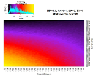Animal research is challenging, and I collected less data than I’d intended my first summer. I instead spent a good chunk of time building a simple model looking at the optimal group composition when individuals vary in their levels of skittishness and the environment varies in its level of predation risk. The heat map on the right is an example output from one of the runs of the model, where warmer colors represent higher average fitness within the group. (Note: you have to be careful not to phrase things in a group selection standpoint when the group is comprised of selfish unrelated individuals.) The model is nowhere near informative enough for publication, but the process itself proved immensely interesting and rewarding, from making me more confident in R to beginning to understand a model’s assumptions and where the output comes from.

During first semester (Fall 2014), I was a TA for an upper-level behavioral ecology course, which was incredibly fun. I had full control of precepts and the students kept me on my toes with their insightful questions. When the lecturer Dr. Costelloe got married during the semester, I stepped in to teach two of the class lectures on game theory and alternative mating tactics. Preparing and delivering the lectures was a great reminder of how much I love science and teaching.

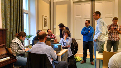October and November were major turning points in my PhD: in October, I attended a fish trajectory analysis workshop at Uppsala University, Sweden. The workshop had a really fantastic group of people, many of whose work I’d read before and whom I was excited to meet. The workshop was the necessary push for me to learn enough R to start analyzing fish data. Once I knew enough coding to visualize tracks and to find answers on Google if I didn’t understand something, my ability to ask and answer questions in R snowballed.

In November, I was able to collect a good chunk of data from pilot experiments for my thesis. These data have felt like a lifeline; for essentially the last year (as of writing this), I’ve analyzed and reanalyzed the trajectories to learn better data analysis and visualization. A crucial insight I had is to look at your data as broadly as you can before zooming in; I spent a month or two puzzling over a 60-FPS 5-minute segment of the tracks before I realized that by reducing the video frame rate to 1 frame per second and looking at the entire hour of the trial, the trend I’d been looking for appeared. The fish trajectories have allowed me to better frame methods for future data collection and to learn the necessary statistics and code for when I have more data.

I attended an animal tracking workshop at Humboldt University, Germany in December with quite a few colleagues from the Princeton EEB, which was a lot of fun. The picture on the left is me giving a brief talk about my work (photo credit: Bernard Chéret). It was really interesting to learn about the fieldwork and network research of the scientists at Humboldt and the discussions were really interesting. Berlin, also, is amazing.

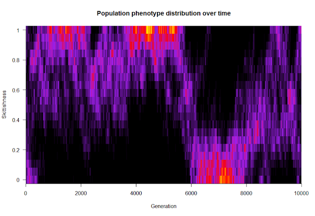
In March, I presented my PhD plans to the department in my second-year talk, and in April I defended those ideas during my generals exam. (More about that time of the PhD here.) Over the summer, I spent a few weeks at the German part of our lab and learned quite a bit of statistics and R from the behavioral ecologists at Max Planck. Separately, I worked on a model regarding the evolutionary dynamics of populations composed of individuals with varying levels of skittishness. The idea was to see what ecological conditions create groups with homogeneous versus heterogeneous membership. The figure below is the distribution of skittishness within the population over time for one run of the model; think of each vertical slice like you’re looking down on a histogram, with warmer colors representing more individuals at that level of skittishness. From this run of the model and for these parameter values, it looks like there are two optima that the population jumps between: everyone is highly skittish (with some noise), or everyone is not skittish.

What I’ve learned from 2nd year

You’re Indiana Jones. Just do it.

Research, by definition, means doing things you’re not sure will work. And you’re right; it probably won’t work the first time you try it. That’s alright. You can’t figure out everything from a distance; don’t be afraid to make mistakes, because that’s how you learn and move forward. Think of it as you’re an adventurer going into the unknown… you’ll have to get your hands dirty.

The PhD is yours. You’re not doing it for anyone else

Grad school is fundamentally different from college in that the work is very isolating. If you’re really at the cutting edge of research, there’s between zero and only a handful of people in the whole world researching your topic. You’re the one who has to provide the justification for why you’re doing what you do, not your advisor or colleagues. Study a topic that makes you happy, and hold yourself to your research standards even when no one’s watching.

Sprinting is no longer feasible. You need a work-life balance.

College is psychologically easier than a PhD because all your checkpoints are defined for you. In grad school, there are almost no checkpoints besides the ones you define yourself. The college-era “work on it ‘til it gets done” mentality is unsustainable in grad school. My first year, I’d work weekends, work until 11pm and then head home, etc. I wasn’t necessarily working smartly at all; I’d just throw time at the problem and be unsatisfied if it wasn’t finished by the time I left. Instead, go home and cook. Jog, see a movie. The time away from work will help you sleep, reinvigorate you when you get back to the office, and likely give you more insights than if you’re always staring at the problem you’re working on. There are always more analyses to do, articles to read, coding to learn, and you can easily spend all your daily mental energy on work. Save some for other things that make you happy!

Reach out to people

Don’t be afraid to ask others for help. Research is hard and you spend a lot of time thinking. You need the occasional anchor of another person’s perspective to say, “Cool idea! What if…” or “Wait, you’re missing this…” It doesn’t reflect poorly on you when you’ve been chewing on a problem for a while and have gotten stuck. Explaining your work to someone else is also a good way to refresh and see the bigger picture of what you’re trying to do. I’ve found that talking to people on the phone or in person is much more efficient for technological hiccups than email.

[Note: the obligatory counterpoint to this advice is to make sure you’ve given the question some legitimate effort before you ask someone else for help! Start the dialogue by introducing the question and detailing what you’ve already tried.]

Think to yourself: “Let me try that…”

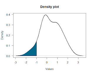Remember: you’re Indiana Jones. Particularly with data analysis, you’re often much more capable of doing something than you’d think. For example, say you have some density plot and you want to shade in a section of it. The R code to do stuff like this is readily available online; you just have to find it and then modify it a bit to suit your needs. [Thanks to R Bloggers for helping me figure out how to do this!]

It’s pretty easy to shade in a part of a normal distribution, so I’ve written code below that lets you shade in any sort of density plot, even weirder-looking ones like the one on the right. Try out the R code below to do it yourself!

R tutorial

Let’s make the distribution. We’ll generate 50 random numbers from a normal distribution with mean 0 and standard deviation 1, then add noise to it. rnorm generates random values from a normal distribution, and runif picks random values between 0 and 1 and adds them to the first distribution. These numbers are now in the variable x.

1
x <- rnorm(50,0,1) + runif(50,0,1)

Let’s now make a density plot of the distribution. A density plot is like a smoothed histogram: it shows what proportion of the data are at that particular value. In the plot above, for example, about 35% of the data have a value around 0. Below, lwd is the line width, and las makes the y-axis labels horizontal. Note that your distribution will look different from the figure above because we’ve picked random values.

1
2
d <- density(x)
plot(d, lwd = 2, main = "Density plot", xlab = "Values", las = 1)

Now we want to shade the region of the distribution from the lowest value up to -1. We make a polygon with two parts: the x- and the y-values. The x values are easy: we just put them between the minimum and -1. The y-values are a bit trickier. We need to find how far into the density distribution (d)’s x values we hit -1, then look at the corresponding y values. The d variable has a lot of information in it, so we’ll use the $ sign to select just the x-values.

1
m <- max(which(d$x <= -1))

This value is the maximum x-value that is less than or equal to -1. To be able to use this value in the code later, we assign it to the variable m.

Now time to make the shaded polygon. The c function means ‘concatenate,’ or to put together. The code below will make coord.x into a vector of values between the minimum x value and -1, with the minimum value and -1 repeated. coord.y will become a vector of the density plot’s y-values from the lowest value (d$y[1]) up to where x = -1 (d$y[m]), along with anchors of 0 at both ends to bring the polygon back to the x-axis. (It sounds complicated but you’ll see that the polygon doesn’t make sense if you don’t include these extra values in coord.x and coord.y.)

1
2
3
4
coord.x <- c(min(d$x), seq(min(d$x), -1, length = m), -1)
coord.y <- c(0, d$y[1:m], 0)

polygon(coord.x, coord.y, col = "deepskyblue4")

Ta-da! A way to make your density plots look fancy for presentations.

Hope this helps. Stay optimistic!

Cheers,
-Matt

EDIT: Since writing this post, I realized that shading the RIGHT side of a threshold in the distribution is quite a bit trickier. Here’s the code to do so:

1
2
3
4
5
6
7
8
9
10
11
12
x <- rnorm(50) + runif(50)
d <- density(x)
plot(d)

# Let's shade everything above zero
m <- min(which(d$x >= 0))
above <- length(d$x) - m + 1   # We do +1 because it's everything > zero

coord.x <- c(0, seq(0, max(d$x), length = above), max(d$x))
coord.y <- c(0, d$y[m:length(d$y)], 0)

polygon(coord.x, coord.y, col = "dodgerblue")