
Intro to data structures
#computer-science #pythonWritten by Matt Sosna on October 19, 2021
Imagine you build a wildly popular app that is quickly growing towards a million users. (Congrats!) While users love the app, they’re complaining that the app is becoming slower and slower, to the point that some users are starting to leave. You notice that the main bottleneck is how user info is retrieved during authentication: currently, your app searches through an unsorted list of Python dictionaries until it finds the requested user ID.
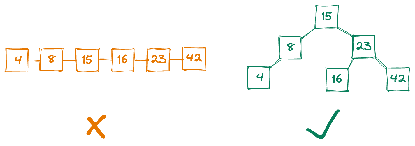
Cursing your 3am self who wrote that code, you wonder how to fix the issue. How can we store user IDs in a way that lets us retrieve any ID as fast as possible? Sorting the list might help, but if we’re searching from the start each time, newer customers with high-numbered IDs will take hundreds of thousands of steps to authenticate. We could start the search from the back of the list, but then customers who’ve been with us from the start would be punished.
A better approach, you realize, is to arrange user data in a binary search tree, which would allow us to find any of our million IDs, on average, in a meager twenty steps. A version of this data structure, indeed, is one of the ways databases index records for lightning-fast retrieval. Quietly migrating user info to a database, your app’s latency drops, everyone is happy, and you vow to never tell anyone about how you originally stored the data.
This example highlights an important point: the data structures our programs use can determine whether our code will scale as the amount of data grows, or whether we’ll need to rewrite everything from scratch every six months. From quickly finding the shortest path between locations, to always serving the highest-priority items in a constantly-changing list, to instantly and securely confirming whether an inputted password is correct, choosing the right data structures is critical for scalable code.
In this post, we’ll cover a few common data structures, discussing their strengths and weaknesses and when they’re used. (A binary search tree is great for indexing databases but bad for generating password hashes, for example.) We’ll implement the structures in Python, then demonstrate some use cases with Leetcode questions.
Even if your daily work never ventures into languages low enough to worry about memory management, you’ll learn how R and Python store your data under the hood. And on a more blunt level, this post will give you foundational knowledge for the coding sections of FAANG tech interviews, if that’s something that interests you!
Table of contents
Getting started
Before we can start playing with any data structures, we need to understand what exactly data structures are and how to compare them. We’ll start by distinguishing the tools (data structures) from their broader purpose (abstract data types) before covering Big O notation, a metric for comparing the speed of operations on data structures. We’ll then quickly go over the fundamental types of data that our data structures store.
Finally, we’ll regularly reiterate that there is no “perfect” data structure. The utility of a data structure is driven entirely by how it is used. It is essential, then, to understand your program’s needs to identify the right tool for the job.
Data structures vs. abstract data types
In programming $-$ as well as in real life! $-$ there are often many ways to accomplish a task. Let’s say, for example, that you want to dig a hole in your backyard. You have at your disposal a pitchfork, hammer, saw, and shovel. Each of these can be thought of as a “data structure” in the sense that they are specific means for accomplishing your task.
But if you separate out the task from how you accomplish the task, you can see that these specific tools are filling the role of “digging tool.” This “digging tool” is your abstract data type: a means of digging. How you actually dig is the data structure. The abstract data type is a theoretical entity, while the data structure is an implementation of that entity.
Here’s another example. Let’s say you want to visit your friend across town. You have at your disposal your bike, car, and feet. Here, the vehicle is the abstract data type: a means of transportation. How you actually travel is the data structure $-$ your bike, car, or feet.
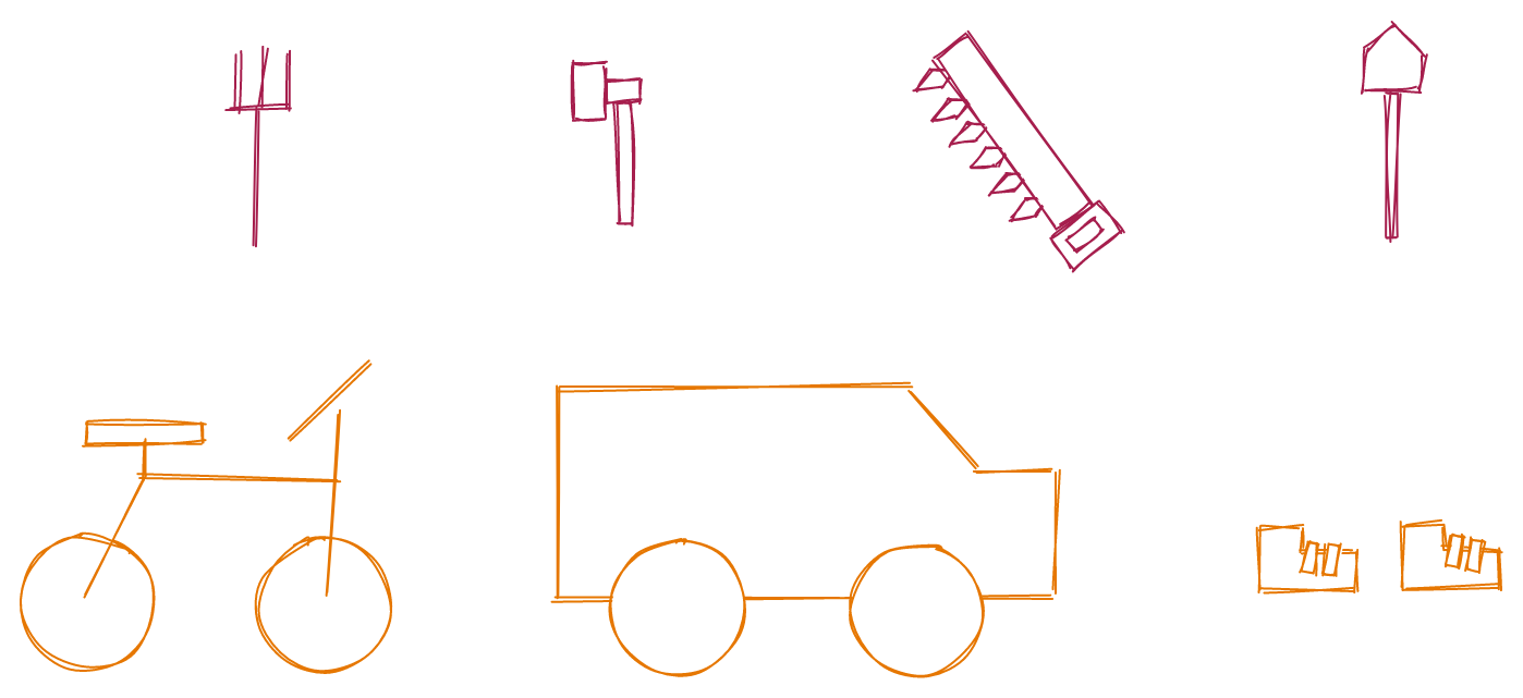
This distinction is important because there are multiple ways to accomplish a task, each with pros and cons that depend on your specific program. In the case of digging a hole, a shovel is the clear winner. But for getting across town, the “right” data structure depends on external context: a car travels the fastest but requires roads, whereas our feet are slow but can traverse tall grass and stairs.
The data structure is what we, the developer, care about, as it’s the specific tool we use to accomplish a task. But our user is only concerned with the abstract data type. Your friend doesn’t care how you get to their house, just that you arrive on time.
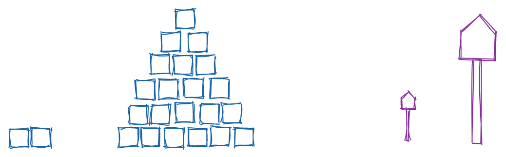
One more example to drive the point home. Imagine you need to put away some clean laundry. A data structure with low write time but high read time would be a pile of clothes on the ground. Adding to this pile is blazing fast, but retrieving any particular item is slow because you have to search through the unsorted pile.
An alternate method would be to neatly arrange your clothes in your dresser and closet. This method would have a high write time but low read time, as it would take longer to put away your clothes, but you’d be able to more quickly access any item you searched for.

While this example might sound silly, it’s actually not too far off from the strategies of dumping data into AWS S3 versus a database, or to some degree storing it in a highly-structured SQL vs. flexible NoSQL database. The dresser and closet isn’t automatically the best approach $-$ transaction logs for an e-commerce store are likely written far more often than read, so a “pile of clothes” approach of saving raw output to S3 can actually work well.
Big O notation
While it makes sense that it’s easier to dig a hole with a shovel than a hammer, how do we quantify the difference in performance? The number of seconds it takes to dig is a good metric, but to deal with holes of differing sizes, we’d probably want something more like seconds per cubic foot.
This only gets us part of the way, though $-$ how do we account for shovels that are different sizes, or the people doing the digging? A bodybuilder with a hammer can dig a hole faster than a toddler with a shovel, but that doesn’t mean the hammer is a better digging tool.
In computer terms, these two considerations can be reframed as the amount of data being processed, and the machine being using. When comparing how well data structures perform some operation $-$ like storing new data or retrieving a requested element $-$ we want a metric that quantifies how performance scales with the amount of data, independent of what machine we use.
To do this, we can turn to Big O notation, denoted as $O(⋅)$. Big O is a measure of the “worst-case” efficiency, an upper bound on how long it would take to accomplish a task (or how much memory it would require, which we won’t cover here). Searching for an element in an unsorted list is $O(n)$, for example, because in the worst case, you have to search the entire list.
Here’s another example of an operation with $O(n)$ time complexity. Printing every element in a Python list takes more time depending on how many elements there are in the list. Specifically, the time it takes grows linearly: if you double the number of elements, you double the time to display all elements.
| Python |
1
2
3
4
# O(n) time complexity
def print_num(arr: list):
    for num in arr:
        print(num)
If we print every pair of elements in the array, meanwhile, our complexity becomes $O(n^2)$. An array of 4 elements requires 16 steps, a 10-element array requires 100 steps, and so on.
| Python |
1
2
3
4
5
# O(n^2) time complexity
def print_pairs(arr: list):
    for num1 in arr:
        for num2 in arr:
            print(num1, num2)
An $O(n^2)$ algorithm isn’t great. Ideally, we want an algorithm that works in constant time, or $O(1)$, where the run time is independent on the amount of data. For example, printing a random value of an array will always take the same time, regardless of the size of the array.
| Python |
1
2
3
# O(1) time
def print_idx(arr: list, i: int):
    print(arr[i])
We can quantify the efficiency of these functions with the %%timeit command in a Jupyter notebook. Below, we already see dramatic increases in the execution time of the $O(n^2)$ print_pairs. We also see the power of the $O(1)$ print_idx, whose execution hovers around 0.153 ms, regardless of the size of the array or whether we’re requesting the first or last element.
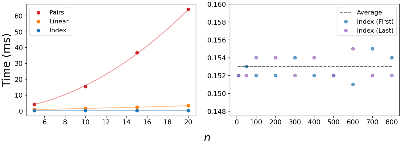
We can use a plot like the one below to compare how algorithms of various efficiencies scale. The green region is ideal $-$ these are the most scalable runtimes, growing at a rate significantly slower than the amount of data. Gray is pretty good, avoid orange if you can, and find any way possible to avoid the red region.
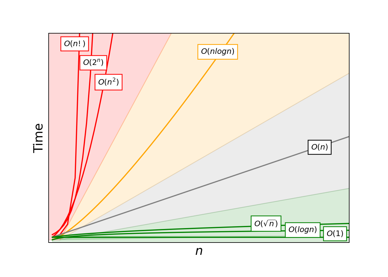
What problems could possibly require an algorithm in the red zone? Red zone algorithms are often necessary for problems where you need to know every possible answer to a question. One example of an $O(2^n)$ algorithm is finding all subsets of an array. Each element in the set can be either 1) included or 2) excluded in a subset. A set of four elements like [A,B,C,D] will therefore have $2^4$, or 16, subsets:
[],[A],[B],[C],[D][A,B],[A,C],[A,D],[B,C],[B,D],[C,D][A,B,C],[A,B,D],[A,C,D],[B,C,D][A,B,C,D]
But an even worse runtime is $O(n!)$. Permutations are a classic example of n-factorial complexity. To find every possible arrangement of [A, B, C, D], we start with one of the four letters in the first position, then one of the remaining three in the second position, and so on. There will therefore be 4 * 3 * 2 * 1, or 24, permutations:
[A,B,C,D],[A,B,D,C],[A,C,B,D],[A,C,D,B],[A,D,B,C],[A,D,C,B][B,A,C,D],[B,A,D,C],[B,C,A,D],[B,C,D,A],[B,D,C,A],[B,D,A,C][C,A,B,D],[C,A,D,B],[C,B,A,D],[C,B,D,A],[C,D,B,A],[C,D,A,B][D,A,B,C],[D,A,C,B],[D,B,A,C],[D,B,C,A],[D,C,A,B],[D,C,B,A]
The runtime of these problems expands at a shocking rate. An array of 10 elements has 1,024 subsets and 3,628,800 permutations. An array of 20 elements has 1,048,576 subsets and 2,432,902,008,176,640,000 permutations!
If your task is specifically to find all subsets or permutations of an inputted array, it’s hard to avoid a $O(2^n)$ or $O(n!)$ runtime. But not all hope is lost if you’re running this operation more than once $-$ there are some architectural tricks you can employ to lessen the burden.[1]
Data types
Finally, we should briefly mention the fundamental data types. If a data structure is a collection of data, what types of data can we have in our structures? There are a few data types universal across programming languages:
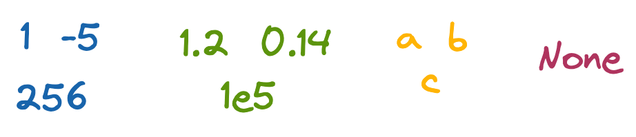
Integers are whole numbers, like 1, -5, and 256. In languages besides Python, you can be more specific with the type of integer, such as signed (+/-) or unsigned (only +), and the number of bits an integer can hold.
Floats are numbers with decimal places, like 1.2, 0.14. In Python, this includes numbers defined with scientific notation, like 1e5. Lower-level languages like C or Java have a related double type, referring to extra precision beyond the decimal place.
Chars are letters, like a, b, c. A collection of them is a string (which is technically an array of chars). The string representations of numbers and symbols, like 5 or ?, are also chars.
Void is a null, like None in Python. Voids explicitly indicate a lack of data, which is a useful default when initializing an array that will be filled, or a function that performs an action but doesn’t specifically return anything (e.g. sending an email).
With abstract data types, Big O notation, and the fundamental data types behind us, let’s get started on the actual data structures! We’ll first cover arrays.
Arrays
Theory
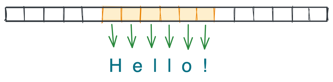
Arrays are one of the most fundamental data structures in computer science, and they come built-in with languages even as low-level as C or Assembly. An array is a group of elements of the same type, like [5, 8, -1] or ['a', 'b', 'c'], located on a contiguous slice of computer memory. Because the array elements are physically next to each another, we can access any index $-$ such as the first, third, or last element $-$ in $O(1)$ time.[2]
Languages like C and Java require specifying an array’s size and data type up front. Python’s list structure is able to circumvent these requirements by storing data as pointers to the elements’ locations in memory (which aren’t necessarily next to each other), and automatically resizing the array when space runs out.
Implementation
We can implement a very basic Array class in Python that mimics the core functionality of arrays in lower-level languages. The main restrictions include:
- Once we’ve allocated space for an array, we can’t get more without creating a new array.
- All values in the array must be the same type.
| Python |
1
2
3
4
5
6
7
8
9
10
11
12
13
14
15
16
17
18
19
20
21
22
from typing import Any

class Array:
    def __init__(self, n: int, dtype: Any):
        self.vals = [None] * n
        self.dtype = dtype

    def get(self, i: int) -> Any:
        """
        Return the value at index i
        """
        return self.vals[i]

    def put(self, i: int, val: Any) -> None:
        """
        Update the array at index i with val. Val must be same type
        as self.dtype
        """
        if not isinstance(val, self.dtype):
            raise ValueError(f"val is {type(val)}; must be {self.dtype}")

        self.vals[i] = val
We can now play around with our Array class. Below, we create an instance, confirm there’s nothing in the first index, fill that slot with a char, then return it. We also confirm that our array rejects a non-char value. It’s not the most exciting code in the world, but it works!
| Python |
1
2
3
4
5
6
7
8
arr = Array(10, str)

arr.get(0)       # None
arr.put(0, 'a')  # None
arr.get(0)       # 'a'

arr.put(1, 5)
# ValueError: val is <class 'int'>; must be <class 'str'>
Example
If you come across a question involving arrays, you’ll most likely want to use Python’s built-in list or a numpy array rather than our Array class. But in the spirit of using an array that doesn’t change size, let’s take on the Leetcode question LC 1089: Duplicate Zeros. The goal of this question is to duplicate all zeros in an array, modifying it in-place so that elements are shifted downstream and popped off, rather than increasing the array size or creating a new one.
| Python |
1
2
3
4
5
6
7
8
9
10
11
12
13
def duplicate_zeros(arr: list) -> None:
    """
    Duplicate all zeros in an array, maintaining the length
    of the original array. e.g. [1, 0, 2, 3] -> [1, 0, 0, 2]
    """
    i = 0

    while i < len(arr):
        if arr[i] == 0:
            arr.insert(i, 0)   # Insert a 0 at index i
            arr.pop()          # Remove the last element
            i += 1
        i += 1
In English, we iteratively move through the list until we find a zero. We then insert another zero and pop off the last element to maintain the array size.
An important detail here is to use a while loop rather than for, as we’re modifying the array as we move through it. The finer control over our index i lets us skip our inserted zero to avoid double-counting.
Linked lists
Theory
Linked lists are another key data structure in computer science. Like arrays, a linked list is a group of values. But unlike arrays, the values in a linked list don’t have to be the same type, and we don’t need to specify the list size ahead of time.
The core element of a linked list is a node, which contains 1) some data, and 2) a pointer to a location in memory. Specifically, any location in memory. Below is a linked list with the values [1, 'a', 0.3] $-$ note how the element sizes differ (four bytes for integers and floats, one byte for chars), each node has a four-byte pointer, the distance between nodes varies, and that the last node contains a null pointer that points off into space.
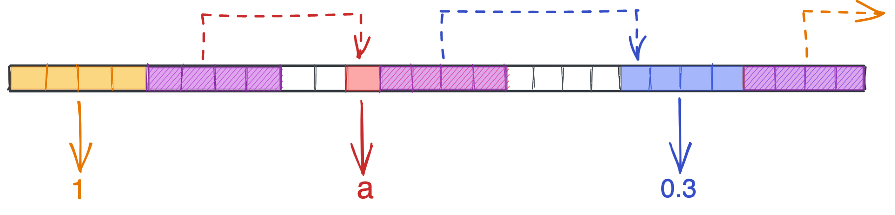
The lack of restrictions on data types and list length make linked lists attractive, but this flexibility comes with a cost. Typically only the head of the list is exposed to a program, meaning we have to traverse the list to find any other node. In other words, we lose that sweet $O(1)$ retrieval for any element besides the first node. If you request the 100th element, it’ll take 100 steps to reach: an $O(n)$ pattern.
We can make our linked lists more versatile by adding pointers to the previous nodes and exposing the tail, or by making the list circular. But overall, choosing linked lists over arrays means paying a cost for flexibility.
Implementation
To create a linked list in Python, we start by defining the node. There are only two pieces we need: the data the node holds, and a pointer to the next node in the list. We also add a __repr__ method to make it easier to see what the node contains.
| Python |
1
2
3
4
5
6
7
class ListNode:
    def __init__(self, val=None, next=None):
        self.val = val
        self.next = next

    def __repr__(self):
        return f"ListNode with val {self.val}"
We can now play around with our ListNode class. Notice how the head of the list is our variable head, and how we have to iteratively append .next to access deeper nodes, since we can’t type an index like [1] or [2] to reach them.
| Python |
1
2
3
4
5
6
7
head = ListNode(5)
head.next = ListNode('abc')
head.next.next = ListNode(4.815162342)

print(head)            # ListNode with val 5
print(head.next)       # ListNode with val abc
print(head.next.next)  # ListNode with val 4.815162342
We can write functions to make it easier to add a node to the end, as well as to the start. We’d do so like this:
| Python |
1
2
3
4
5
6
7
8
9
10
def add_to_end(head: ListNode, val: Any) -> None:
    ptr = head
    while ptr.next:
        ptr = ptr.next
    ptr.next = ListNode(val)

def add_to_front(head: ListNode, val: Any) -> ListNode:
    node = ListNode(val)
    node.next = head
    return node
In add_to_end, we create a variable called ptr (“pointer”) that starts at head and traverses the list until it reaches the last node, whose .next attribute is a null pointer. We then simply set that node’s .next value to a new ListNode. We don’t need to return anything for our change to take effect.
add_to_front is simpler: we create a new head, then set its .next pointer to the head of our existing linked list. However, we need to manually update head outside our function with this new node, because otherwise head still points to the old head.
| Python |
1
2
3
4
5
6
7
8
9
10
11
12
13
14
15
16
17
# Create and extend list
head = ListNode(5)
add_to_end(head, 'abc')
add_to_end(head, 4.815162342)

# Print the contents
print(head)            # ListNode with val 5
print(head.next)       # ListNode with val abc
print(head.next.next)  # ListNode with val 4.815162342

# Try to update head
add_to_front(head, 0)
print(head)            # ListNode with val 5

# Correctly update head
head = add_to_front(head, 0)
print(head)            # ListNode with val 0
Examples
One common question with linked lists is to return the middle node. Because we typically only have the head of the list, there’s no way for us to know ahead of time how long the list is. On first glance, it might therefore seem like we’d need to traverse the list twice: once to find how long the list is, and then again to go halfway.
But there’s actually a clever way to find the middle with one pass. Before, we used a pointer to traverse the list one node at a time until we reached the end. But what if we had two pointers, one moving one node at a time and the other two at a time? When the fast pointer reached the end of the list, our slow pointer would be at the middle.
Here’s how we’d answer LC 876: Middle of Linked List.
| Python |
1
2
3
4
5
6
7
8
9
10
11
12
13
14
15
def find_middle(head: ListNode) -> ListNode:
    """
    Return middle node of linked list. If even number of nodes,
    returns the second middle node.
    """
    # Set slow and fast pointers
    slow = head
    fast = head.next

    # Traverse the list
    while fast and fast.next:
        slow = slow.next
        fast = fast.next.next

    return slow
Whenever I work on Leetcode questions, I like to draw out examples and make sure I’m doing what I think I’m doing. For example, it can be hard to remember if we should initialize fast to head or to head.next. If you draw out a simple list where you know what the middle should be, you can quickly confirm that head.next is the right option.
1
2
3
4
5
6
7
8
9
10
# List: A -> B -> C -> D -> E
# Middle: C

# Start at head: incorrect
# Slow: A -> B -> C -> D  ==> Middle: D
# Fast: A -> C -> E -> null

# Start at head.next: correct
# Slow: A -> B -> C       ==> Middle: C
# Fast: B -> D -> null
LC 141: Linked List Cycle is another example of using slow and fast pointers. The idea here is to determine whether the list has a cycle, which occurs when a node’s next pointer points to an earlier node in the list.
Traversing this list will continue forever, as we will never exit the cycle. A first guess might be to set some threshold on how long our traversal is running, or on how many repeated patterns we’ve seen over some time period, but a simpler approach is to again use two pointers.
We can’t use while fast and fast.next anymore, since this evaluates to False only when we’ve reached the end of the list. Rather, we’ll again instantiate slow and fast to the first and second nodes, then move them through the list at different speeds until they match. If we reach the end of the list, we return False; if the two pointers ever point to the same node, we return True.
| Python |
1
2
3
4
5
6
7
8
9
10
11
12
13
14
15
16
17
def has_cycle(head: ListNode) -> bool:
    """
    Determines whether a linked list has a cycle
    """
    slow = head
    fast = head.next

    while slow != fast:

        # Reach end of list
        if not (fast or fast.next):
            return False

        slow = slow.next
        fast = fast.next.next

    return True
Trees
Theory
Trees extend the idea of a linked list by allowing for nodes to have more than one “next” node. Tree nodes can have one, two, or many child nodes, allowing for data to be represented in a flexible branching pattern. By setting rules on how data is organized, we can store and retrieve data very efficiently.
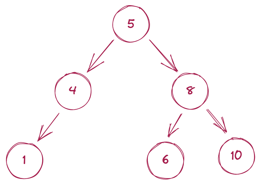
One type of tree is a binary search tree (BST); at the start of this post we briefly mentioned how efficiently BSTs can retrieve data. This efficiency stems from two important rules governing a BST’s structure:
- A node can have at most two children.
- Every node in the left subtree must contain a smaller value, and every node in the right subtree must contain a larger value.
Searching for a value in a BST takes at worst $O(log\ n)$ time[3], meaning we can find a requested value among millions or even billions of records very rapidly. Let’s say we’re searching for the node with the value x. We can use the following algorithm to quickly find this node in a BST.
- Start at the root of the tree.
- If x = the node value: stop.
- If x < the node value: go to the left child.
- If x > the node value: go to the right child.
- Go to Step 2.
If we’re unsure whether the requested node exists in the tree, we just modify steps 3 and 4 to stop the search if we try to access a child that doesn’t exist.
Implementation
Creating a TreeNode is nearly identical to creating a ListNode. The only difference is that rather than one next attribute, we have left and right attributes, which refer to the left and right children of the node. (If we’re defining a tree with more than two children, we can name these attributes child1, child2, child3, etc.)
| Python |
1
2
3
4
5
6
7
8
class TreeNode:
    def __init__(self, val=None, left=None, right=None):
        self.val = val
        self.left = left
        self.right = right

    def __repr__(self):
      return f"TreeNode with val {self.val}"
We can then create a tree with three levels as such. Note that this tree is just a binary tree, not a BST, as the values aren’t sorted.
| Python |
1
2
3
4
5
6
7
8
9
10
11
12
13
14
15
16
17
18
19
# Level 0
root = TreeNode('a')

# Level 1
root.left = TreeNode('b')
root.right = TreeNode('c')

# Level 2
root.left.left = TreeNode('d')
root.left.right = TreeNode('e')

root.right.left = TreeNode('f')
root.right.right = TreeNode('g')

#            a
#          /   \
#         b     c
#        / \   / \
#       d   e f   g
Examples
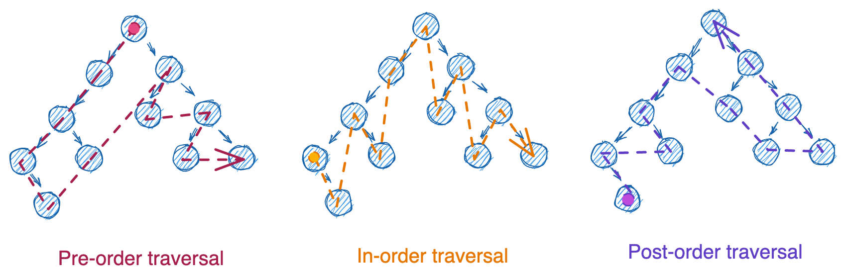
Questions involving binary trees often center on different ways of traversing the nodes. Traversal typically begins at the root node and then follows a set of steps for processing each node and its children. But the order in which nodes are processed depends entirely on the order in which we process the parent relative to the children: before (pre-order), in between the left and right (in-order), or after (post-order). Each of the traversals below started at the root node, but the order that nodes were processed differed entirely.
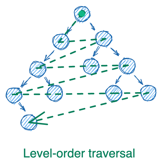
These three types of traversal can occur with iteration (using a while loop and a stack) or with recursion (using a function that calls itself). There’s also a fourth type of traversal, level-order, which utilizes a queue. We won’t cover stacks and queues in this post, but just think of them as lists where you can only remove from the end (stacks) or the start (queues).
The patterns for the first three types of traversals are nearly identical, so we’ll just choose in-order traversal. Below we code out the iterative and recursive methods for LC 94: Binary Tree Inorder Traversal, starting with the iterative version.
| Python |
1
2
3
4
5
6
7
8
9
10
11
12
13
14
15
16
17
18
19
20
21
# Iterative traversal
def traverse_in_order(root: TreeNode) -> List[int]:
    """
    Traverse a binary tree, returning list of values in order
    """
    answer = []
    stack = [(root, False)]   # (node, whether visited yet)

    while stack:
        node, visited = stack.pop()

        if node:

            if visited:
                answer.append(node.val)
            else:
                stack.append((node.right, False))
                stack.append((node, True))
                stack.append((node.left, False))

    return answer
In English, we perform these steps:
- Lines 6-7: Instantiate a list for our answer (
answer) and a stack (stack) that contains a tuple of our root node andFalseindicating that we haven’t visited this node yet. - Line 9: Start a
whileloop, which executes as long as any elements exist instack. - Lines 10-12: Remove the last element of the stack with
.pop, then check ifnodeexists.- (
nodewon’t always exist in later iterations for nodes with no children).
- (
- Lines 14-15: If
nodeexists and we’ve visited this node before, append our node value to the answer. - Lines 16-19: If we haven’t visited this node yet, add its right child (with a flag saying we haven’t seen it yet), the current node (with a flag seeing we have seen it already), and then the left child with a “haven’t seen yet” flag.
- Lines 9-19: Repeat steps 3-6 until we’ve processed all nodes.
- Line 21: Return a list of node values sorted in-order.
The way we append nodes to the stack (lines 17-19) might seem out of order $-$ shouldn’t the left node come first? But because stacks are Last In First Out, the first node we want to process needs to be the last node we add to the stack. Hence we add right first, then left.
Now for the recursive method:
| Python |
1
2
3
4
5
6
7
8
9
10
11
12
13
14
15
16
17
18
19
20
21
22
# Recursive traversal
class Solution:
    def __init__(self):
        self.answer = []

    def traverse_inorder(self, root: TreeNode) -> List[Any]:
        """
        Traverse a binary tree, returning list of values in-order
        """
        self._traverse(root)
        return self.answer

    def _traverse(self, node: Optional[TreeNode]) -> None:
      """
      Recursive function for in-order traversal
      """
        if not node:
            return None

        self._traverse(node.left)
        self.answer.append(node.val)
        self._traverse(node.right)
In English, we perform these steps:
- Lines 2-4: Create a class that initializes with a list for our answer (
self.answer). - Lines 6-11: Define a function,
traverse_inorder, which takes the root node of a tree, calls the recursive function_traverse, and then returnsself.answer. - Lines 13-22: Define a recursive function
_traversethat takes in a node. The function checks ifnodeexists before calling itself on the node’s left child, appending the node’s value toself.answer, and then calling itself on the node’s right child.
How do we change from in-order to pre-order or post-order? For both methods, we simply rearrange the order in which node is processed relative to its children. The rest of the code remains unchanged.
| Python |
1
2
3
4
5
6
7
8
9
10
11
12
13
# Change to pre-order traversal
def iterative(root):
    ...
    stack.append((node.right, False))
    stack.append((node.left, False))
    stack.append((node, True))     # <- change
    ...

def _traverse(self, node):
    ...
    self.answer.append(node.val)   # <- change
    self._traverse(node.left)
    self._traverse(node.right)
Graphs
Theory
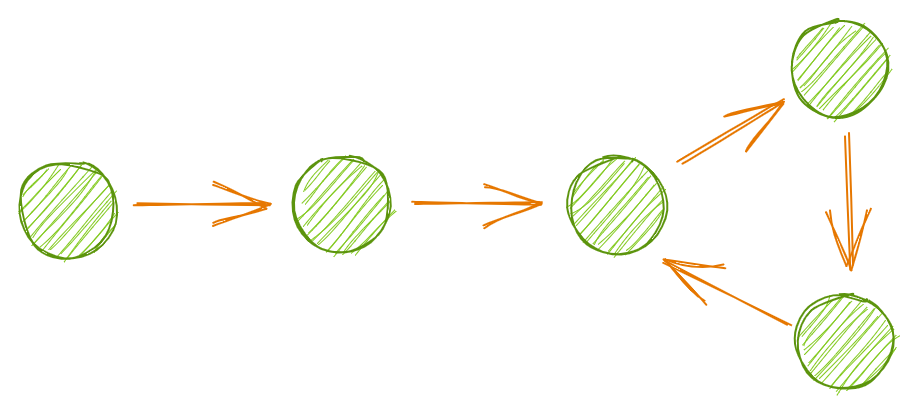
Trees expand the scope of linked lists by allowing for more than one child per node. With graphs, we expand scope again by loosening trees’ strict parent-child relationship. The nodes in a graph have no explicit hierarchy, and any node can be connected to any other node.
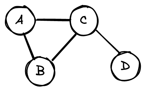
Graphs are usually represented as adjacency matrices. The above graph, for example, would have the following matrix.
\[\begin{bmatrix} 0 & 1 & 1 & 0\\ 1 & 0 & 1 & 0\\ 1 & 1 & 0 & 1\\ 0 & 0 & 1 & 0 \end{bmatrix}\]Each row and column represent a node. A 1 at row $i$ and column $j$, or $A_{ij}=1$, represents a connection between node $i$ and node $j$. $A_{ij}=0$ means nodes $i$ and $j$ aren’t connected.
None of the nodes in this graph are connected to themselves, meaning the matrix diagonal is 0. Similarly, $A_{ij} = A_{ji}$ because connections are undirected: if A is connected to B, then B is connected to A. As a result, the adjacency matrix is symmetric along the diagonal.
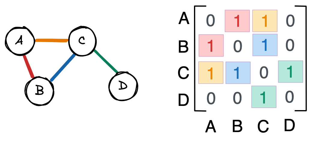
I find a bunch of 1s and 0s in a matrix a little hard to interpret, so here’s that same graph and matrix with colors.
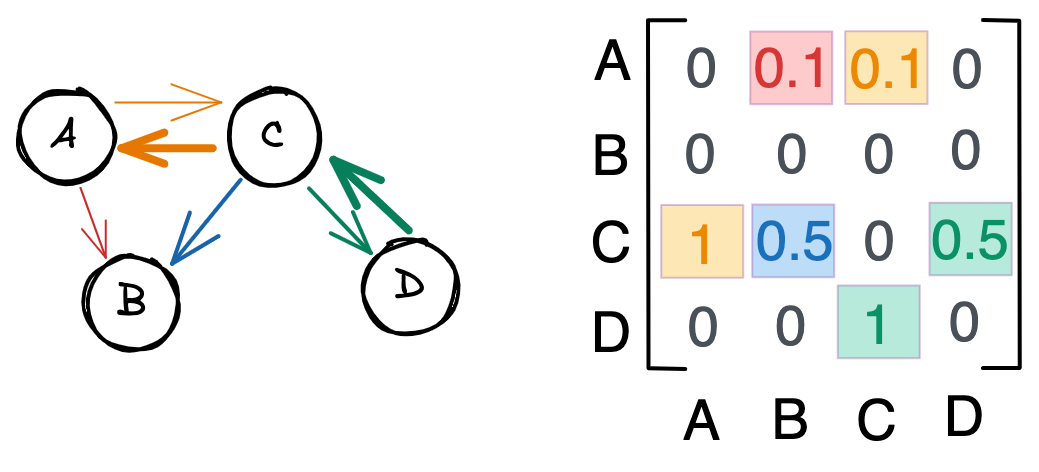
A weighted graph with directed edges would look something like this. Notice how the relationships are no longer symmetric $-$ the second row in the adjacency matrix is now empty, for example, because $B$ has no outbound connections. We also have numbers that range between 0 and 1, which reflect the strength of the connection. For example, $C$ feeds into $A$ more strongly than $A$ feeds into $C$.
Implementation
For simplicity, let’s implement a graph that is unweighted and undirected. The main structure in our class is a list of lists: each list is a row, with the indices in the list representing columns. Instantiating a Graph object requires specifying the number of nodes, n, to create our list of lists. We can then access a connection between nodes a and b with self.graph[a][b].
| Python |
1
2
3
4
5
6
7
8
9
10
11
12
13
14
15
16
17
18
19
20
21
from typing import List

class Graph:
    def __init__(self, n: int):
        self.graph = [[0]*n for _ in range(n)]

    def connect(self, a: int, b: int) -> List[List[int]]:
        """
        Updates self.graph to connect nodes A and B.
        """
        self.graph[a][b] = 1
        self.graph[b][a] = 1
        return self.graph

    def disconnect(self, a: int, b: int) -> List[List[int]]:
        """
        Updates self.graph to disconnect nodes A and B.
        """
        self.graph[a][b] = 0
        self.graph[b][a] = 0
        return self.graph
We can recreate the graph in the first example in this section like this:
| Python |
1
2
3
4
5
6
7
8
9
10
11
g = Graph(4)

# A's connections
g.connect(0, 1)
g.connect(0, 2)

# B's connections (not included by A)
g.connect(1, 2)

# C's connections (not included by B)
g.connect(2, 3)
Example
One trickier graph question is identifying the number of connected components, or sub-clusters, within a graph. In the below graph, for example, we can identify three distinct components.
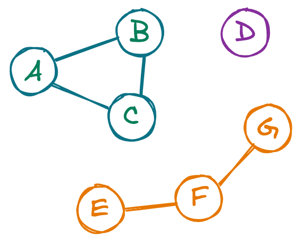
To answer LC 323: Number of Connected Components, we’ll examine each node in the graph, visiting its neighbors, its neighbors’ neighbors, and so on, until we only encounter nodes we’ve already seen. We’ll then check if there are any nodes in the graph that we haven’t visited $-$ if any exist, that means there’s at least one more cluster, so we grab a new node and repeat the process.
| Python |
1
2
3
4
5
6
7
8
9
10
11
12
13
14
15
16
17
18
19
20
21
22
23
24
25
26
27
28
29
30
31
32
33
34
35
def get_n_components(self, mat: List[List[int]]) -> int:
    """
    Given an adjacency matrix, returns the number of connected
    components
    """
    q = []
    unseen = [*range(len(mat))]

    answer = 0

    while q or unseen:

        # If all neighbors exhausted, traverse a new cluster
        if not q:
            q.append(unseen.pop(0))
            answer += 1

        # Pick a node from the current cluster
        focal = q.pop(0)
        i = 0

        # Search through all remaining nodes for connections
        while i < len(unseen):
            node = unseen[i]

            # If node connected to focal, add node to queue
            # to search through its neighbors, and remove
            # from unseen nodes to avoid infinite loop
            if mat[focal][node] == 1:
                q.append(node)
                unseen.remove(node)
            else:
                i += 1

    return answer
In English:
- Lines 5-8: Instantiate a queue (
q), list of nodes (unseen), and number of components (answer). - Line 10: Start a
whileloop that executes as long as there are either nodes to be processed in the queue, or nodes we haven’t visited yet. - Lines 13-15: If the queue is empty, remove the first node from
unseenand increment the number of components. - Lines 18-19: Pick the next available node in the queue (
focal). - Line 22: Start a
whileloop that executes as long as we haven’t processed all remaining nodes. - Line 23: Name the node we’re currently on to make the next lines more readable.
- Line 28-30: If the node we’re on is connected to
focal, add it to our queue of nodes in the current cluster, and remove it from our list of nodes that could be in another cluster (unseen). - Lines 31-32: If the node we’re on isn’t connected to
focal, continue onto the next potential node.
Hash tables
Theory
Let’s finish this post with one more foundational data structure: the hash table, also called hash map.[4] When we moved on from arrays, we left behind the enviable $O(1)$ retrieval time to gain flexibility in data types and array size. But what if we could get that lightning-fast efficiency again, even for data that differ in type and memory location?
This is where hash tables come in. Data in these tables are associated with key-value pairs $-$ input the key, and a hash function takes you to the associated value in $O(1)$ time. Hash tables actually use an array of pointers to achieve this speed; the job of the hash function is to identify the index in the array that holds the pointer to a key’s value.
Below is how our linked list from earlier would look as a hash table. The green box is our table, which stores the keys key1, key2, and key3. When a user passes in one of these keys to the table, the key is sent through the hash function to find an index in the array of pointers (purple). That pointer then takes us to the area in memory storing the actual value. Each pointer in our array is four bytes, while the size of the values they point to can vary.
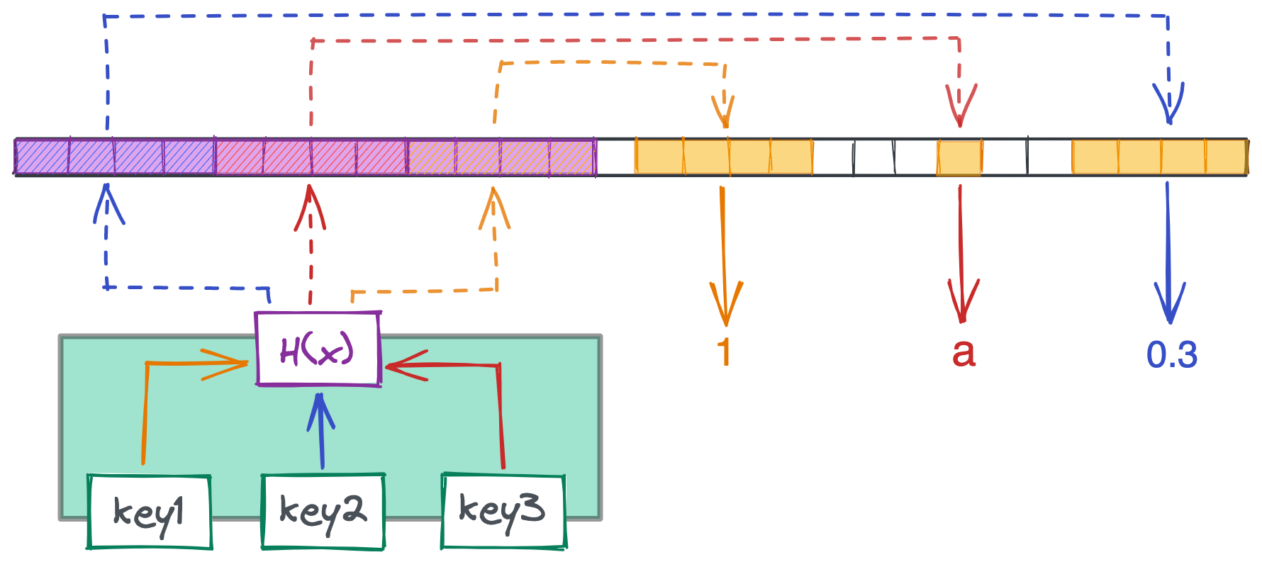
The main workhorse of the table is the hash function, which maps an input to an output within some range. Python’s hash function, for example, outputs values between -9,223,372,036,854,775,808 and 9,223,372,036,854,775,807. We then bucket the hashed value $-$ often by dividing by the length of our array and taking the remainder $-$ to return an index in our array of pointers. In the above example, the output would be 0, 1, or 2: the indices of the pointer array.
Since our array won’t have infinite indices, it’s possible $-$ and even likely $-$ that two distinct inputs will receive the same hashed output. This collision would mean that two inputs, like user IDs 1005778 and 9609217, would both land on the pointer that returns Jane Reader, even if they’re separate users. We don’t want that!
The first fix is to ensure our hash function distributes outputs uniformally. Each array index should have an equal probability of being selected $-$ if certain indices are more likely than others, we’ll run into collisions more frequently than we need to.
A more involved solution involves bringing in another data structure: linked lists. Rather than having each pointer point to an exact value in memory, each pointer could instead point to a linked list. If we tried saving a new key-value pair where the hashed key collides with an existing key, we’d simply append another node to the list at that location in memory. Add a little logic for traversing the list and knowing when to stop, and you’re good to go!
But collisions also aren’t inherently bad $-$ sometimes we want different inputs to receive the same output. If your cool app from the start of this post has four servers handling traffic, you could use a basic hash function like the one below to balance the load among your servers.
| Python |
1
2
3
4
5
6
7
8
9
10
def choose_server_for_request(request_id: int) -> int:
  """
  Returns the server ID (0, 1, 2, or 3) to send a request to.
  """
  return hash(str(request_id)) % 4

choose_server_for_request(2877448)   # Sends to server 2
choose_server_for_request(2877449)   # Sends to server 1
choose_server_for_request(2877450)   # Sends to server 3
choose_server_for_request(2877451)   # Sends to server 0
Implementation
Hash maps might sound similar to Python dictionaries, and indeed the Python dict is a hash table! But if we had to create one from scratch, we could do so like below.
| Python |
1
2
3
4
5
6
7
8
9
10
11
12
13
14
15
16
17
18
19
20
21
22
23
24
25
26
27
28
29
30
31
32
33
34
35
36
37
38
39
class HashTable:
    def __init__(self, n_slots: int):
        self.array = [[] * n_slots]

    def put(self, key: str, value: Any) -> bool:
        """
        Saves a key-value pair to the corresponding list in
        self.array. If key-value pair already present, updates
        key's value.
        """
        slot = self._calculate_slot(key)

        # Update value if key already present
        for k, v in self.array[slot]:
            if k == key:
                v = value
                return True

        # Otherwise add a new tuple
        self.array[slot].append((key, value))
        return True

    def get(self, key: str) -> Any:
        """
        Retrieves a key-value pair. Raises error if key not present.
        """
        slot = self._calculate_slot(key)

        for k, v in self.array[slot]:
            if key == k:
                return v

        raise ValueError(f"key {key} not present.")

    def _calculate_slot(self, key: str) -> int:
        """
        Return the corresponding list in self.array.
        """
        return hash(key) % len(self.array)
To deal with hash collisions, we use a list of lists for self.array, then traverse the list when retrieving or adding values. We store both the key and value in our list to be able to identify the key-value pair we’re looking for, given that multiple keys will have the same array index.
Below, we implement a very basic login system. We hash user passwords before they’re stored in self.array[slot], meaning that even if the passwords were stolen, the time it would take to crack them might give users enough time to change them. (This excellent video by Computerphile is a deep dive on this, and it should motivate you to never use a password like password!)
| Python |
1
2
3
4
5
6
7
8
9
10
11
12
13
14
15
16
17
# Create our hash table
ht = HashTable(3)

# User registers with email and password
email = 'omar@example.com'
password = 'password'
ht.put(key=email, value=hash(password))

# View hashed password
ht.get(email)  # 2710932929137326597

# Login attempts
wrong_password = '12345678'
right_password = 'password'

hash(wrong_password) == ht.get(email)  # False
hash(right_password) == ht.get(email)  # True
Example
To finish off this post, let’s answer the classic Leetcode problem LC 1: Two Sum. Like we did with arrays, we’ll just use the Python built-in class (dict). The question is as follows: given an array of integers and a target, return the indices of two array elements that sum to the target. Assume there is only one answer. With the array [1, 2, 3] and target 4, for example, we’d return [0, 2], as 1 + 3 = 4.
There are multiple approaches to this problem, humorously outlined in this parody of a technical interview. The first is to brute force compare every pair of numbers (e.g. 1+2, 1+3, 2+3), which will definitely work but will take $O(n^2)$ time. A better approach is to sort the array and then use two pointers, one at the start and one at the end, and iteratively move the left or right pointer if their sum is less than or greater than the target, respectively. This approach takes $O(nlogn)$ time due to sorting.
But we can actually achieve $O(n)$ time, visiting each element at most once, by using a hash map. The key concept here is that for each number num, we need to see if there’s some other number that equals target-num. We can use a Python dictionary (i.e. hash map) to store numbers we’ve already seen, then use that sweet $O(1)$ lookup time to see if we’ve already seen a number that matches target-num. If there’s a match, we return the indices of the two numbers.
| Python |
1
2
3
4
5
6
def two_sum(arr: List[int], target: int) -> List[int]:
    seen = {}
    for i, num in enumerate(arr):
      	if target-num in seen:
            return [i, seen[target-num]]
        seen[num] = i
Here’s how this would look for our array [1, 2, 3] with target 4. Here we write out the logic for each iteration of the for loop.
| Python |
1
2
3
4
5
6
7
8
9
10
11
12
13
14
# seen = {}
# num: 1
# target - num: 4 - 1 = 3
# 3 not in seen; continue

# seen = {1: 0}
# num: 2
# target - num: 4 - 2 = 2
# 2 not in seen; continue

# seen = {1: 0, 2: 1}
# num: 3
# target - num: 4 - 3 = 1
# 1 in seen; return indices [2, 0]
Conclusions
This post took on the humble task of introducing data structures, the ways that programming languages store data. We started by distinguishing the task (abstract data type) from the implementation (data structure), using Big O notation to quantify the efficiency of operations on data structures, and finally the types of data we store in our structures. We then covered the theory of arrays, linked lists, trees, graphs, and hash maps, as well as implemented each in Python and answered a Leetcode question or two.
Despite how massive this post is, there’s still plenty to learn about data structures. Trees, for example, can be reshaped to solve dozens of use cases, such as representing two-dimensional space, autocompleting inputted strings, quickly running calculations on interval data, and more. Check out this page for some advanced structures and their common use cases if you’re interested.
Finally, it’s important to again distinguish data structures from abstract data types. We didn’t cover stacks, queues, or heaps in this post, as there are multiple ways to implement each. A stack, for example, can be implemented with an array or linked list depending on your needs. Keep an eye on upcoming post on some of these more common abstract data types.
That’s it for now. See you next time!
Best,
Matt
Footnotes
1. Big O notation
We probably can’t do much for the first user to request all permutations for a specific array. But we can store the array and its answer in a hash table. For every subsequent user, we can check our table to see if that array has already been queried. (We’d want to sort the array, remove nulls, etc. that would otherwise make identical arrays look different.) If a user requests an array whose permutations have already been computed, we could respond with a lightning fast $O(1)$ runtime. If not… back to $O(n!)$.
This concept is called caching, or memoizing. Here’s what that would look like in Python.
| Python |
1
2
3
4
5
6
7
8
9
10
11
12
13
14
15
16
17
18
19
20
21
22
23
24
25
26
27
28
29
30
31
class PermutationCalculator:
    """
    Methods for calculating permutations
    """
    def __init__(self):
        self.seen = {}

    def get_permutations(self, arr: list) -> list:
        """"
        Returns permutations of list, first checking self.seen.
        """
        # Ensure [A, B, null], [null, B, A], etc. are treated the same
        clean_str = self._sort_and_remove_nulls(arr)

        # Don't perform calculation if we've seen it before!
        if clean_str in self.seen:
            return self.seen[clean_str]

        # If new request, do the hard work
        result = self._permute(clean_str)

        # Cache the result for instant retrieval next time
        self.seen[clean_str] = result

        return result

    def _sort_and_remove_nulls(self, arr: list) -> str:
        ...

    def _permute(self, clean_str: str) -> list:
        ...
Another approach is dynamic programming, which involves recursively breaking down a problem into as small a piece as possible, then caching the results of the pieces. For example, if our question was modified slightly to return the number of permutations, rather than the actual permutations, it could be helpful to cache values like $5!$ or $10!$ to avoid having to calculate them each time.
2. Theory
Array indexing takes $O(1)$ time because there are always only three steps required:
- Go to the location in memory of the start of the array
- Identify the type of data in the array (e.g. float)
- Return the value in memory at
array start+index * (size of data type)
The type of data is important because data types differ in how much memory they require. A char is one byte, for example, while an int is four. Getting the element at index 3 means traversing three bytes from the start for a string, while traversing twelve bytes for an array of integers.
Step 3 hints at why so many programming languages are 0-indexed: the first element of an array is 0 elements away from the start. Returning that value, then, is easy if index * (size of data type) is zero and we can just return the value at array start.
3. Theory
Note that $O(logn)$ is $log_2$, not $log_{10}$ or the natural log. This pattern is easy to see in a binary tree, as with every step we take in our search, we reduce the remaining nodes to search by half.
4. Theory
This Stack Overflow post is a good explanation for the difference between hash maps and hash tables. A hash map is technically an abstract data type, but the terms are used largely interchangeably.