
Intermediate SQL
#sqlWritten by Matt Sosna on January 17, 2022
When I started learning SQL, I found it hard to progress beyond the absolute basics. I loved DataCamp’s courses because I could just type the code directly into a console on the screen. But once the courses ended, how could I practice what I learned? And how could I continue improving, when all the tutorials I found just consisted of code snippits, without an underlying database I could query myself?
I found myself in a “chicken or egg” problem – I needed access to databases to learn enough SQL to get hired, but the only databases I was aware of were at those companies where I was trying to get hired!
It turns out it’s straightforward to create your own database to play with. In this post, we’ll create a simple relational database that will let us explore SQL topics beyond the basics. If you understand the below query, then you’re prepared for the rest of this post. (And if not, check out the SQL primer in the engineering essentials post and the SQL vs. NoSQL deep dive.)
| SQL |
1
2
3
4
5
6
7
8
9
10
11
12
SELECT
    s.id AS student_id,
    g.score
FROM
    students AS s
LEFT JOIN
    grades AS g
    ON s.id = g.student_id
WHERE
    g.score > 90
ORDER BY
    g.score DESC;
Table of contents
Setting up
When learning a new language, practice is critical. It’s one thing to read this post and nod along, and another to be able to explore ideas on your own. So let’s start by setting up a database on your computer so you can experiment and practice. While it sounds intimidating, it’ll actually be straightforward!
The first step is to install SQL on your computer. We’ll use PostgreSQL (Postgres), a common SQL dialect. To do so, we visit the download page, select our operating system (e.g. Windows), and then run the installation. If you set a password on your database, keep it handy for the next step! (Since our database won’t be public, it’s fine to use a simple password like admin.)

The next step is to install pgAdmin, a graphical user interface (GUI) that makes it easy to interact with our PostgreSQL database(s). We do this by going to the installation page, clicking the link for our operating system, and then following the steps.
(As an FYI, this tutorial uses Postgres 14 and pgAdmin 4 v6.3.)
Once both have been installed, we open pgAdmin and click on “Add new server.” This step actually sets up a connection to an existing server, which is why we needed to install Postgres first. I named my server home and passed in the password I defined during the Postgres installation.
We’re now ready to create some tables! Let’s make a set of tables that describe the data a school might have: students, classrooms, and grades. We’ll model our data such that a classroom consists of multiple students, each with multiple grades.
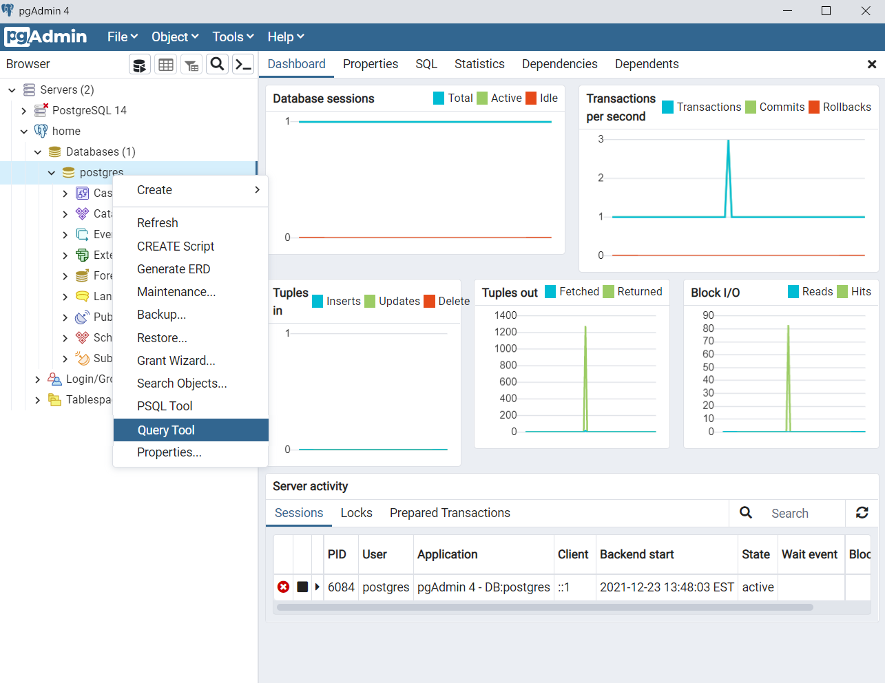
We could do all this with the GUI, but we’ll instead write code to make our workflow repeatable. To write the queries that will create our tables, we’ll right click on postgres (under home > Databases (1) > postgres) and then click on Query Tool.
Let’s start by creating the classrooms table. We’ll keep this table simple: it’ll just consist of an id and the teacher name. Type the following code into the query tool and hit run.
| SQL |
1
2
3
4
5
6
DROP TABLE IF EXISTS classrooms CASCADE;

CREATE TABLE classrooms (
    id INT PRIMARY KEY GENERATED ALWAYS AS IDENTITY,
    teacher VARCHAR(100)
);
In the first line, DROP TABLE IF EXISTS classrooms, deletes the classrooms table if it already exists. (Makes sense!) Postgres will stop us from deleting classrooms if other tables point to it, so we specify CASCADE to override this constraint.[1] This is ok – if we’re deleting classrooms, we’re probably regenerating everything from scratch, so all the other tables are getting deleted too!
Adding DROP TABLE IF EXISTS before CREATE TABLE lets us codify our database schema in a script, which is handy if we decide to change our database in some way down the road – add a table, change the datatype of a column, etc. We can simply store the instructions for generating our database in a script, update that script when we want to make a change, and then rerun it.[2]
We’re also now able to version control our schema and share it. In fact, the entire database in this post can be recreated from this script, so feel free to experiment!
Line 4 may also catch your eye: here we specify that id is the primary key, meaning each row must contain a value in this column, and that each value must be unique. To avoid needing to keep track of which id values have already been used, we use GENERATED ALWAYS AS IDENTITY, an alternative to the sequence syntax. As a result, when inserting data into this table, we only need to provide the teacher names.
Finally, on line 5 we specify that teacher is a string with a maximum length of 100 characters.[3] If we come across a teacher whose name is longer than this, we’ll have to either abbreviate their name or alter the table.
Let’s now create the students table. Our table will consist of a unique id, the student’s name, and a foreign key that points to classrooms.
| SQL |
1
2
3
4
5
6
7
8
9
10
DROP TABLE IF EXISTS students CASCADE;

CREATE TABLE students (
    id INT PRIMARY KEY GENERATED ALWAYS AS IDENTITY,
    name VARCHAR(100),
    classroom_id INT,
    CONSTRAINT fk_classrooms
        FOREIGN KEY(classroom_id)
        REFERENCES classrooms(id)
);
We again drop the table if it exists before creating it, then specify an auto-incrementing id and a 100-character name. We now include a classroom_id column, and on lines 7-9 specify that this column points to the id column of the classrooms table.
By specifying that classroom_id is a foreign key, we’ve set a rule on how data can be written to students. Postgres won’t allow us to insert a row into students with a classroom_id that doesn’t exist in classrooms.
| SQL |
1
2
3
4
5
6
7
8
9
10
11
12
INSERT INTO students
    (name, classroom_id)
VALUES
    ('Matt', 1);

/*
ERROR: insert or update on table "students" violates foreign
    key constraint "fk_classrooms"
DETAIL: Key (classroom_id)=(1) is not present in table
    "classrooms".
SQL state: 23503
*/
So let’s now create some classrooms. Since we specified that the id column will be automatically incremented for us, we only have to insert the teacher names.
| SQL |
1
2
3
4
5
6
7
8
9
10
11
12
13
14
INSERT INTO classrooms
    (teacher)
VALUES
    ('Mary'),
    ('Jonah');

SELECT * FROM classrooms;

/*
 id | teacher
 -- | -------
  1 | Mary
  2 | Jonah
*/
Great! Now that we have some classrooms, we can add records to students and reference these classrooms.
| SQL |
1
2
3
4
5
6
7
8
9
10
11
12
13
14
15
16
INSERT INTO students
    (name, classroom_id)
 VALUES
    ('Adam', 1),
    ('Betty', 1),
    ('Caroline', 2);

SELECT * FROM students;

/*
 id | name     | classroom_id
 -- | -------- | ------------
  1 | Adam     |            1
  2 | Betty    |            1
  3 | Caroline |            2
*/
What happens if we get a student who hasn’t yet been assigned a classroom? Do we have to wait for them to receive a classroom before we can record them in the database?
The answer is no: while our foreign key requirement will block writes that reference non-existing IDs in classrooms, it allows us to pass in a NULL for classroom_id. We can do this by explicitly stating NULL for classroom_id or by only passing in name.
| SQL |
1
2
3
4
5
6
7
8
9
10
11
12
13
14
15
16
17
18
19
20
21
22
23
-- Explicitly specify NULL
INSERT INTO students
    (name, classroom_id)
VALUES
    ('Dina', NULL);

-- Implicitly specify NULL
INSERT INTO students
    (name)
VALUES
    ('Evan');

SELECT * FROM students;

/*
 id | name     | classroom_id
 -- | -------- | ------------
  1 | Adam     |            1
  2 | Betty    |            1
  3 | Caroline |            2
  4 | Dina     |       [null]
  5 | Evan     |       [null]
*/
Finally, let’s record some grades. Since grades correspond to assignments – such as homework, projects, attendance, and exams – we’ll actually use two tables to store our data more efficiently. assignments will contain data on the assignments themselves, while grades will record how each student performed on the assignments.
| SQL |
1
2
3
4
5
6
7
8
9
10
11
12
13
14
15
16
17
18
19
20
21
22
23
DROP TABLE IF EXISTS assignments CASCADE;
DROP TABLE IF EXISTS grades CASCADE;

CREATE TABLE assignments (
    id INT PRIMARY KEY GENERATED ALWAYS AS IDENTITY,
    category VARCHAR(20),
    name VARCHAR(200),
    due_date DATE,
    weight FLOAT
);

CREATE TABLE grades (
    id INT PRIMARY KEY GENERATED ALWAYS AS IDENTITY,
    assignment_id INT,
    score INT,
    student_id INT,
    CONSTRAINT fk_assignments
        FOREIGN KEY(assignment_id)
        REFERENCES assignments(id),
    CONSTRAINT fk_students
        FOREIGN KEY(student_id)
        REFERENCES students(id)
);
Rather than insert rows by hand, though, let’s now upload the data through CSV’s. You can download the files from this repo or write them yourselves. Note that to allow pgAdmin to access the data you might need to update the permissions on the folder (db_data below).
| SQL |
1
2
3
4
5
6
7
8
9
10
11
12
13
14
15
16
17
COPY assignments(category, name, due_date, weight)
FROM 'C:/Users/mgsosna/Desktop/db_data/assignments.csv'
DELIMITER ','
CSV HEADER;
/*
COPY 5
Query returned successfully in 118 msec.
*/

COPY grades(assignment_id, score, student_id)
FROM 'C:/Users/mgsosna/Desktop/db_data/grades.csv'
DELIMITER ','
CSV HEADER;
/*
COPY 25
Query returned successfully in 64 msec.
*/
Finally, let’s take a look to make sure everything’s in place. The query below finds the average score on each assignment category, grouped by teacher.
| SQL |
1
2
3
4
5
6
7
8
9
10
11
12
13
14
15
16
17
18
19
20
21
22
23
24
25
26
27
28
SELECT
    c.teacher,
    a.category,
    ROUND(AVG(g.score), 1) AS avg_score
FROM
    students AS s
INNER JOIN classrooms AS c
    ON c.id = s.classroom_id
INNER JOIN grades AS g
    ON s.id = g.student_id
INNER JOIN assignments AS a
    ON a.id = g.assignment_id
GROUP BY
    1,
    2
ORDER BY
    3 DESC;

/*
 teacher | category  | avg_score
 ------- | --------- | ---------
 Jonah   |  project  |     100.0
 Jonah   |  homework |      94.0
 Jonah   |  exam     |      92.5
 Mary    |  homework |      78.3
 Mary    |  exam     |      76.0
 Mary    |  project  |      69.5
*/
Good work setting up a database! We’re now ready to experiment with some trickier SQL concepts. We’ll start with syntax you might not have come across yet that’ll give you finer control over your queries. We’ll then cover some other joins and ways to organize your queries as they grow into the dozens or hundreds of lines.
Useful syntax
Filters: WHERE vs. HAVING
You’re likely familiar with the WHERE filter, and you might have heard of HAVING. But how exactly do they differ? Let’s perform some queries on grades to find out.
First, let’s sample some rows from grades to remind ourselves what the data look like. We use ORDER BY RANDOM() to shuffle the rows, then LIMIT to take 5. (Ordering all the rows in a table just to get a sample is pretty inefficient, but it’s fine if the table is small.)
| SQL |
1
2
3
4
5
6
7
8
9
10
11
12
13
14
15
16
17
18
SELECT
    *
FROM
    grades
ORDER BY
    RANDOM()
LIMIT
    5;

/*
 id | assignment_id | score | student_id
 -- | ------------- | ----- | ----------
 14 |             4 |   100 |          3
 22 |             2 |    91 |          5
 23 |             3 |    85 |          5
 16 |             1 |    81 |          4
  9 |             4 |    64 |          2
*/
Each row is a student’s score on an assignment. Now, let’s say we want to know each student’s average score. We’d perform a GROUP BY, using AVG(score) and rounding to keep things tidy.
| SQL |
1
2
3
4
5
6
7
8
9
10
11
12
13
14
15
16
17
18
19
SELECT
    student_id,
    ROUND(AVG(score),1) AS avg_score
FROM
    grades
GROUP BY
    student_id
ORDER BY
    student_id;

/*
 student_id | avg_score
 ---------- | ---------
          1 |      80.8
          2 |      70.4
          3 |      94.6
          4 |      79.6
          5 |      83.4
*/
Now, let’s say we want the above table but only with rows where avg_score is between 50 and 75. In other words, we only want to show student 2. What happens if we use a WHERE filter?
| SQL |
1
2
3
4
5
6
7
8
9
10
11
12
13
14
15
16
17
18
19
20
SELECT
    student_id,
    ROUND(AVG(score),1) AS avg_score
FROM
    grades
WHERE
    score BETWEEN 50 AND 75
GROUP BY
    student_id
ORDER BY
    student_id;

/*
 student_id | avg_score
 ---------- | ---------
          1 |      75.0
          2 |      70.4
          3 |      64.0
          4 |      67.0
*/
That doesn’t look right at all. Student 5 correctly disappeared, but students 1, 3, and 4 are still there. Worse, their avg_score values changed! This would probably cause some panic if these numbers were going into an important report and you didn’t understand what happened.
What we actually want to do is use a HAVING filter. See the difference below.
| SQL |
1
2
3
4
5
6
7
8
9
10
11
12
13
14
15
16
17
SELECT
    student_id,
    ROUND(AVG(score),1) AS avg_score
FROM
    grades
GROUP BY
    student_id
HAVING
    ROUND(AVG(score),1) BETWEEN 50 AND 75
ORDER BY
    student_id;

/*
 student_id | avg_score
 ---------- | ---------
          2 |      70.4
*/
These two queries return dramatically different results because WHERE and HAVING filter data at different stages of the aggregation. The WHERE query above filters the data before the aggregation, while HAVING filters the results.
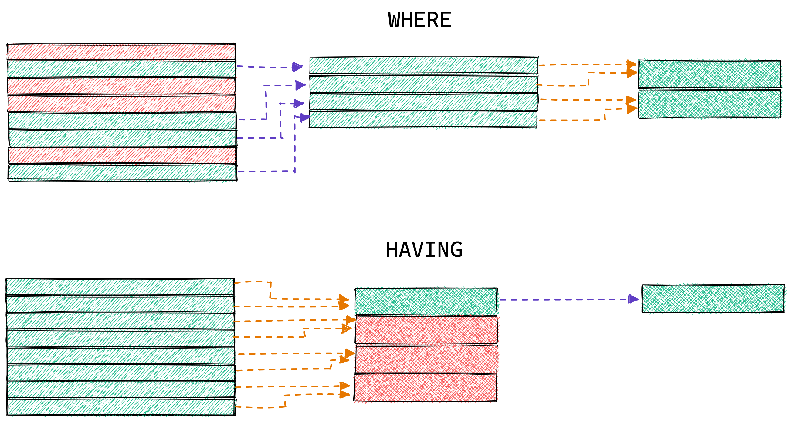
The aggregation results in the WHERE query above changed because we changed the raw data used to calculate each student’s average score. Student 5 didn’t have any scores between 50 and 75 and was therefore dropped. The HAVING query, meanwhile, just filtered the results after the calculation.
Once you’re comfortable with WHERE and HAVING, you can use both to create very specific queries, for example finding students whose average homework score was between 50 and 75.
| SQL |
1
2
3
4
5
6
7
8
9
10
11
12
13
14
15
16
17
18
19
20
SELECT
    student_id,
    ROUND(AVG(score),1) AS avg_score
FROM
    grades AS g
INNER JOIN
    assignments AS a
    ON a.id = g.assignment_id
WHERE
    a.category = 'homework'
GROUP BY
    student_id
HAVING
    ROUND(AVG(score),1) BETWEEN 50 AND 75;

/*
 student_id | avg_score
 ---------- | ---------
          2 |      74.5
*/
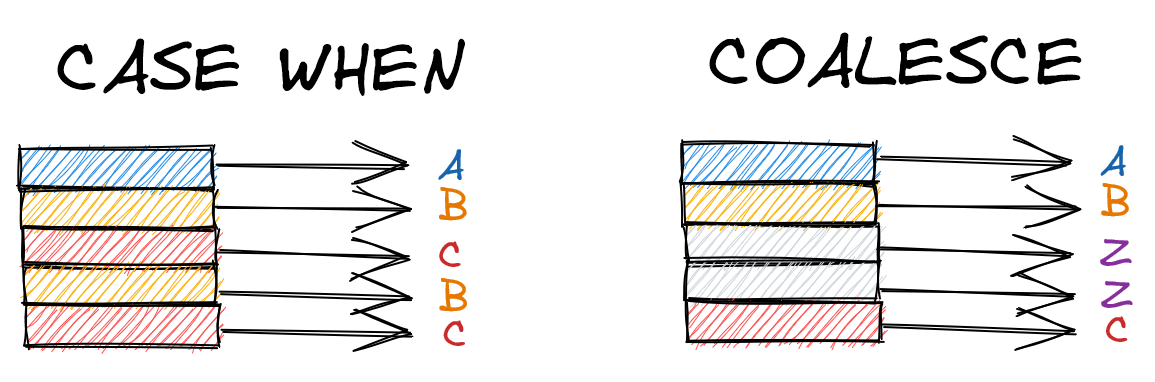
If-then: CASE WHEN & COALESCE
It’s common to need some kind of if-else logic on a column. Maybe you have a table of model predictions, for example, and you want to binarize the values into positive and negative labels by some threshold.
In our database, let’s say we want to convert the scores from our grades table into letter grades. We can easily do so with CASE WHEN.
| SQL |
1
2
3
4
5
6
7
8
9
10
11
12
13
14
15
16
17
18
19
20
21
SELECT
    score,
    CASE
        WHEN score < 60 THEN 'F'
        WHEN score < 70 THEN 'D'
        WHEN score < 80 THEN 'C'
        WHEN score < 90 THEN 'B'
        ELSE 'A'
    END AS letter
FROM
    grades;

/*
 score | letter
 ----- | ------
    82 | B
    82 | B
    80 | B
    75 | C
   ... | ...
*/
The logic we pass into CASE WHEN can extend to multiple columns. We can generate an instructor column from our students table, for example, that has the student’s teacher if available, otherwise their own name.
| SQL |
1
2
3
4
5
6
7
8
9
10
11
12
13
14
15
16
17
18
19
20
21
22
SELECT
    name,
    teacher,
    CASE
        WHEN teacher IS NOT NULL THEN teacher
        ELSE name
    END AS instructor
FROM
    students AS s
LEFT JOIN
    classrooms AS c
    ON c.id = s.classroom_id;

/*
 name     | teacher | instructor
 -------- | ------- | ----------
 Adam     | Mary    | Mary
 Betty    | Mary    | Mary
 Caroline | Jonah   | Jonah
 Dina     | [null]  | Dina
 Evan     | [null]  | Evan
*/
If all we’re doing is handling nulls, though, COALESCE is a cleaner choice. COALESCE returns the first non-null value among the arguments passed into it. Rewriting the above query, we get this:
| SQL |
1
2
3
4
5
6
7
8
9
10
11
12
13
14
15
16
17
18
19
SELECT
    name,
    teacher,
    COALESCE(teacher, name)
FROM
    students AS s
LEFT JOIN
    classrooms AS c
    ON c.id = s.classroom_id;

/*
 name     | teacher | instructor
 -------- | ------- | ----------
 Adam     | Mary    | Mary
 Betty    | Mary    | Mary
 Caroline | Jonah   | Jonah
 Dina     | [null]  | Dina
 Evan     | [null]  | Evan
*/
Nice and clean! Line 4 above is the same as lines 4-7 in the second CASE WHEN example: if teacher is non-null, return that value. Otherwise return name.
COALESCE will move down the arguments you provide until it finds a non-null value. If all values are nulls, it returns null.
| SQL |
1
2
3
4
5
6
7
8
9
10
11
12
13
14
15
SELECT
    COALESCE(NULL, NULL, NULL, 4);
/*
 coalesce
 --------
        4
 */

 SELECT
    COALESCE(NULL);
/*
 coalesce
 --------
 [null]
 */
Finally, there is an IF statement in Postgres, but it’s used for control flow on multiple queries rather than within one. It’s unlikely you’ll be using IF much as a data scientist – even as a data engineer, I’d imagine you’d handle such logic in a coordinator like Airflow, so we’ll skip it here.[4]
Set operators: UNION, INTERSECT, and EXCEPT
When we JOIN tables, we append data horizontally. In the below query, for example, we bring together Adam’s data from the students, grades, and assignments tables, creating a table with those columns side by side.
| SQL |
1
2
3
4
5
6
7
8
9
10
11
12
13
14
15
16
17
18
19
20
21
22
23
24
SELECT
    s.name,
    g.score,
    a.category
FROM
    students AS s
INNER JOIN
    grades AS g
    ON s.id = g.student_id
INNER JOIN
    assignments AS a
    ON a.id = g.assignment_id
WHERE
    s.name = 'Adam';

/*
 name | score | category
 ---- | ----- | --------
 Adam |    82 | homework
 Adam |    82 | homework
 Adam |    80 | exam
 Adam |    75 | project
 Adam |    85 | exam
*/
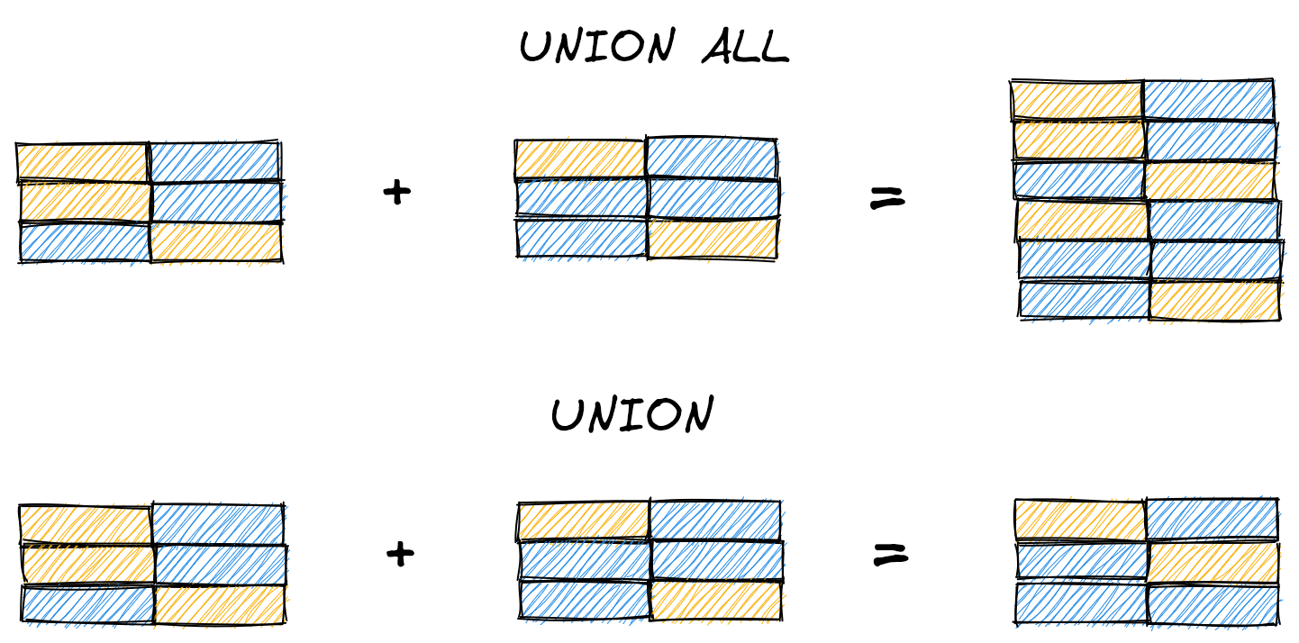
Horizontally appending our data serves us well most of the time. But what if we want to stack query results vertically?
Let’s imagine that our school is incredibly corrupt and uses students’ names to determine whether they graduate, not their grades. Students pass if their names either 1) start with A or B, or 2) are five letters long. We can find all graduating students by finding students that meet each criterion, then using UNION ALL to stack the rows on top of each other.
| SQL |
1
2
3
4
5
6
7
8
9
10
11
12
13
14
15
16
17
18
19
20
21
22
23
24
25
26
27
28
29
30
31
32
33
SELECT
    *
FROM (
    SELECT
        name,
        'Name starts with A/B' as reason
    FROM
        students
    WHERE
        LEFT(name,1) IN ('A', 'B')
) AS x

UNION ALL

SELECT
    *
FROM (
    SELECT
        name,
        'Name is 5 letters long' AS reason
    FROM
        students
    WHERE
        LENGTH(name) = 5
) AS y;

/*
 name  | reason
 ----  | ------
 Adam  | Name starts with A/B
 Betty | Name starts with A/B
 Betty | Name is 5 letters long
*/
We’ve now seen our first subqueries, the building blocks for more complex queries, on lines 4-11 and 18-24. Notice that these subqueries need to be named (x and y) for UNION ALL to work.
You may also notice that we used UNION ALL instead of UNION. The distinction is that UNION ALL returns all rows, whereas UNION removes duplicates (including within x and y). The results are identical for this query because Betty meets both criteria, but if we didn’t include the reason column, we’d only see Betty once with UNION.
| SQL |
1
2
3
4
5
6
7
8
9
10
11
12
13
14
15
16
17
18
19
20
21
22
23
24
25
26
27
28
29
30
SELECT
    *
FROM (
    SELECT
        name  -- <- No `reason` column
    FROM
        students
    WHERE
        LEFT(name,1) IN ('A', 'B')
) AS x

UNION  -- <- Now UNION, not UNION ALL

SELECT
    *
FROM (
    SELECT
        name  -- <- No `reason` column
    FROM
        students
    WHERE
        LENGTH(name) = 5
) AS y;

/*
 name
 -----
 Adam
 Betty   <- Duplicate Betty dropped because UNION
*/
Choosing UNION or UNION ALL depends on how you want to handle duplicates. When writing complex queries, I prefer using UNION ALL to make sure the resulting table has the number of rows I expect – if there are duplicates, I’ve likely messed up a JOIN somewhere earlier. Your query will be far more performant if you fix the issue at the source, rather than filtering at the end.
UNION and UNION ALL are set operators that return all rows from subqueries A and B (sans duplicates with UNION). Two other operators, INTERSECT and EXCEPT, let us return only rows that meet certain criteria. INTERSECT only returns rows present in both subqueries, while EXCEPT returns rows in A that are not in B.
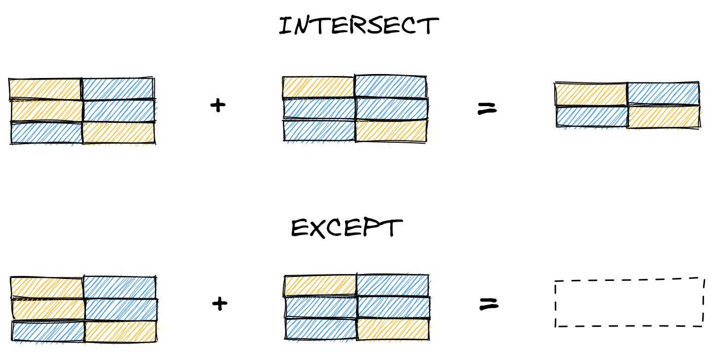
Here we demonstrate INTERSECT, which finds the rows shared between the subqueries (i.e. rows with IDs 2 or 3). Unlike with UNION, we don’t need to name the subqueries.
| SQL |
1
2
3
4
5
6
7
8
9
10
11
12
13
14
15
16
17
18
19
20
21
22
SELECT
    *
FROM
    students
WHERE
    id IN (1,2,3)

INTERSECT

SELECT
    *
FROM
    students
WHERE
    id IN (2,3,4);

/*
 id | name     | classroom_id
 -- | -------- | ------------
  2 | Betty    |            1
  3 | Caroline |            2
*/
And here we show the same query but with EXCEPT, which finds the rows in A that are not in B (i.e. rows with ID 1).
| SQL |
1
2
3
4
5
6
7
8
9
10
11
12
13
14
15
16
17
18
19
20
21
SELECT
    *
FROM
    students
WHERE
    id IN (1,2,3)

EXCEPT

SELECT
    *
FROM
    students
WHERE
    id IN (2,3,4);

/*
 id | name     | classroom_id
 -- | -------- | ------------
  1 | Adam     |            1
*/
Together, set operators give us the power to combine query results (UNION), view overlapping records (INTERSECT), and see precisely which rows differ between tables (EXCEPT). No more printing out the tables to stack or manually compare them!
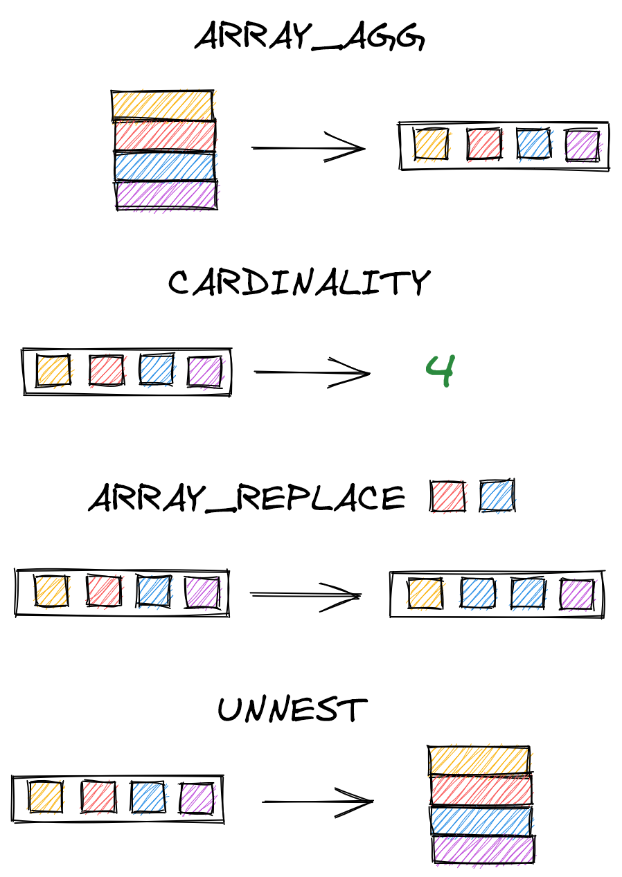
Array functions
Data in relational databases is usually atomic, where each cell contains one value (e.g. one score per row in the grades table). But sometimes storing values as an array can be useful. For this type of data, Postgres offers a wide range of array functions that let us create and manipulate arrays.
One useful function is ARRAY_AGG, which converts rows into an array. Below, we combine ARRAY_AGG(score) with GROUP BY name to create arrays of all scores for each student.
| SQL |
1
2
3
4
5
6
7
8
9
10
11
12
13
14
15
16
17
18
19
20
21
22
SELECT
    name,
    ARRAY_AGG(score) AS scores
FROM
    students AS s
INNER JOIN
    grades AS g
    ON s.id = g.student_id
GROUP BY
    name
ORDER BY
    name;

/*
 name     | scores
 -------- | ------
 Adam     | {82,82,80,75,85}
 Betty    | {74,75,70,64,69}
 Caroline | {96,92,90,100,95}
 Dina     | {81,80,84,64,89}
 Evan     | {67,91,85,93,81}
*/
We can use CARDINALITY to find the length of an array, and ARRAY_REPLACE to replace specified values. (Alternatively, ARRAY_REMOVE removes them.)
| SQL |
1
2
3
4
5
6
7
8
9
10
11
12
13
14
15
16
17
18
19
20
21
22
23
24
SELECT
    name,
    ARRAY_AGG(score) AS scores,
    CARDINALITY(ARRAY_AGG(score)) AS length,
    ARRAY_REPLACE(ARRAY_AGG(score), 82, NULL) AS replaced
FROM
    students AS s
INNER JOIN
    grades AS g
    ON s.id = g.student_id
GROUP BY
    name
ORDER BY
    name;

/*
 name     | scores            | length | replaced
 -------- | ----------------- | ------ | --------------------
 Adam     | {82,82,80,75,85}  |      5 | {NULL,NULL,80,75,85}
 Betty    | {74,75,70,64,69}  |      5 | {74,75,70,64,69}
 Caroline | {96,92,90,100,95} |      5 | {96,92,90,100,95}
 Dina     | {81,80,84,64,89}  |      5 | {81,80,84,64,89}
 Evan     | {67,91,85,93,81}  |      5 | {67,91,85,93,81}
*/
One last function you may find useful is UNNEST, which unpacks an array to rows. (It is, in essence, the opposite of ARRAY_AGG.)
| SQL |
1
2
3
4
5
6
7
8
9
10
11
SELECT
    'name' AS name,
    UNNEST(ARRAY[1, 2, 3]);

/*
 name  | unnest
 ----  | ------
 name  |      1
 name  |      2
 name  |      3
*/
Great! Having covered filters, if-then logic, set operators, and array functions, let’s now move on to constructing more advanced queries.
Advanced queries
Self joins
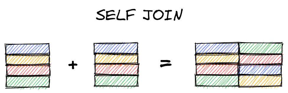
Occasionally, we may want to join our table with itself to get the data we need. One common example is the “manager” problem, which we’ll rephrase here as the “best friend” problem. The idea is that if rows in a table contain values pointing to other rows in the table (such as IDs), then we can join the table to itself to get additional data corresponding to those values.
Let’s start by adding and then populating a best_friend_id column to our students table.
| SQL |
1
2
3
4
5
6
7
8
9
10
11
12
13
14
15
16
17
18
19
20
21
22
23
24
25
26
27
28
29
30
31
32
33
34
ALTER TABLE students
ADD best_friend_id INT;

UPDATE students
SET best_friend_id = 5
WHERE id = 1;

UPDATE students
SET best_friend_id = 4
WHERE id = 2;

UPDATE students
SET best_friend_id = 2
WHERE id = 3;

UPDATE students
SET best_friend_id = 2
WHERE id = 4;

UPDATE students
SET best_friend_id = 1
WHERE id = 5;

SELECT * FROM students;

/*
 id  | name     | classroom_id | best_friend_id
 --- | -------- | ------------ | --------------
   1 | Adam     |            1 |              5
   2 | Betty    |            1 |              4
   3 | Caroline |            2 |              2
   4 | Dina     |       [null] |              2
   5 | Evan     |       [null] |              1
*/
Storing the identity of the best friend as a number is efficient but not very readable. To identify who each student’s best friend is, we perform a self join. We join students to itself, where the id column in one table is the best_friend_id in the other. We distinguish the tables with aliases, x and y in our example.
| SQL |
1
2
3
4
5
6
7
8
9
10
11
12
13
14
15
16
17
18
SELECT
    x.name,
    y.name AS best_friend
FROM
    students AS x
INNER JOIN
    students AS y
    ON y.id = x.best_friend_id;

/*
 name     | best_friend
 -------- | -----------
 Adam     | Evan
 Betty    | Dina
 Caroline | Betty
 Dina     | Betty
 Evan     | Adam
*/
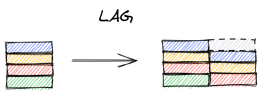
Window functions
Window functions are similar to aggregation functions (anything with a GROUP BY) in that they apply a calculation to a grouped set of values. Unlike aggregation functions, however, window functions don’t reduce the number of rows.
Let’s say we take the average score for each student. On lines 4-6 below, we add the OVER and PARTITION BY to convert the aggregation into a window function.
| SQL |
1
2
3
4
5
6
7
8
9
10
11
12
13
14
15
16
17
18
19
20
21
22
23
24
SELECT
    s.name,
    g.score,
    AVG(g.score) OVER (
        PARTITION BY s.name
    )
FROM
    students AS s
INNER JOIN
    grades AS g
    ON s.id = g.student_id;

/*
 name  | score | avg
 ------| ----- | ----------
 Adam  |    82 | 80.8000...
 Adam  |    82 | 80.8000...
 Adam  |    80 | 80.8000...
 Adam  |    75 | 80.8000...
 Adam  |    85 | 80.8000...
 Betty |    74 | 70.4000...
 Betty |    75 | 70.4000...
 ...   |   ... |        ...
*/
For aggregators like AVG, MIN, or MAX, each row in the PARTITION BY grouping will have the same value. This might prove useful for some analyses, but it doesn’t really exemplify the strength of window functions.
A more useful case is ranking each student’s scores. First, here’s how we’d rank scores across all students. We use RANK() OVER, then pass in the column to rank.
| SQL |
1
2
3
4
5
6
7
8
9
10
11
12
13
14
15
16
17
18
19
20
SELECT
    s.name,
    g.score,
    RANK() OVER (
        ORDER BY g.score
    )
FROM
    grades AS g
INNER JOIN
    students AS s
    ON s.id = g.student_id;

/*
 name  | score | rank
 ----- | ----- | ----
 Betty |    64 |    1
 Dina  |    64 |    1
 Evan  |    67 |    3
 ...   |   ... |  ...
*/
Ranking scores by each student is a one-line change: we simply add PARTITION BY s.name to the OVER clause.
| SQL |
1
2
3
4
5
6
7
8
9
10
11
12
13
14
15
16
17
18
19
20
21
22
23
24
25
26
27
28
29
30
SELECT
    s.name,
    g.score,
    RANK() OVER (
        PARTITION BY s.name  -- ranks by student
        ORDER BY g.score
    )
FROM
    grades AS g
INNER JOIN
    students AS s
    ON s.id = g.student_id;

/*
 name     | score | rank
 -------- | ----- | ----
 Adam     |    75 |    1
 Adam     |    80 |    2
 Adam     |    82 |    3
 Adam     |    82 |    3
 Adam     |    85 |    5
 Betty    |    64 |    1
 Betty    |    69 |    2
 Betty    |    70 |    3
 Betty    |    74 |    4
 Betty    |    75 |    5
 Caroline |    90 |    1
 Caroline |    92 |    2
 ...      |   ... |  ...
*/
Other window functions include calculating leading and lagging values (e.g. the previous value of a time series), the cumulative distribution, and dense or percent ranks.
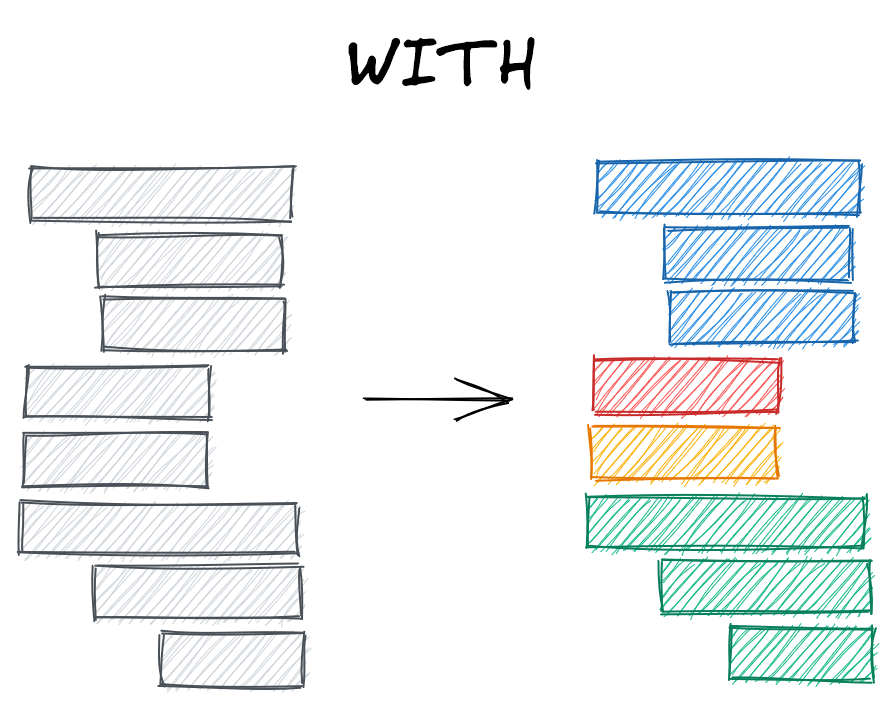
WITH
Let’s end this section by covering a technique that will empower us to write queries as complex as we can imagine, simply by stringing together subqueries. WITH lets us name a subquery, meaning we can then reference that subquery’s results elsewhere.
Let’s say, for example, that we want to label whether students’ scores in grades are higher than their average score. Knocking this out in one query seems straightforward – we just need to calculate each average with a GROUP BY and then do something like g.score > avg, right? Let’s start with the GROUP BY aggregation.
| SQL |
1
2
3
4
5
6
7
8
9
10
11
12
13
14
15
16
17
18
19
20
SELECT
    s.name,
    ROUND(AVG(g.score),1) AS avg
FROM
    students AS s
INNER JOIN
    grades AS g
    ON s.id = g.student_id
GROUP BY
    s.name;

/*
 name     | avg
 -------- | ----
 Dina     | 79.6
 Evan     | 83.4
 Betty    | 70.4
 Caroline | 94.6
 Adam     | 80.8
*/
Easy enough. But how do we then compare the individual scores to those averages? Both attempts below raise an error.
| SQL |
1
2
3
4
5
6
7
8
9
10
11
12
13
14
SELECT
    s.name,
    ROUND(AVG(g.score),1) AS avg,
    g.score > avg
    ...
    -- ERROR: column "avg" does not exist

SELECT
    s.name,
    ROUND(AVG(g.score),1) AS avg,
    g.score > ROUND(AVG(g.score),1)
    ...
    -- ERROR: column "g.score" must appear in the GROUP BY
    -- clause or be used in an aggregate function
We can get this to work by calling a window function twice, but it looks a little ugly.
| SQL |
1
2
3
4
5
SELECT
    s.name,
    AVG(g.score) OVER (PARTITION BY s.name),
    g.score > AVG(g.score) OVER (PARTITION BY s.name)
    ...
A cleaner and more scalable alternative is to use WITH. We can break our query into two subqueries – one to calculate the averages, and one to join that table of averages into grades.
| SQL |
1
2
3
4
5
6
7
8
9
10
11
12
13
14
15
16
17
18
19
20
21
22
23
24
25
26
27
28
29
30
31
32
33
34
35
36
37
WITH averages AS (
    SELECT
        s.id,
        ROUND(AVG(g.score),1) AS avg_score
    FROM
        students AS s
    INNER JOIN
        grades AS g
        ON s.id = g.student_id
    GROUP BY
        s.id
)
SELECT
    s.name,
    g.score,
    a.avg_score,
    g.score > a.avg_score AS above_avg
FROM
    students AS s
INNER JOIN
    grades AS g
    ON s.id = g.student_id
INNER JOIN
    averages AS a
    ON a.id = s.id;

/*
 name  | score | avg_score | above_avg
 ----- | ----- | --------- | ---------
 Adam  |    82 |      80.8 | true
 Adam  |    82 |      80.8 | true
 Adam  |    80 |      80.8 | false
 Adam  |    75 |      80.8 | false
 Adam  |    85 |      80.8 | true
 Betty |    74 |      70.4 | true
 Betty |    75 |      70.4 | true
*/
The WITH query is substantially longer than just writing the window function twice. Why bother? Well, this more verbose query provides two important advantages: scalability and readability.
Queries can become ridiculously long – at Meta (Facebook), the longest query I’ve come across (so far!) was over 1000 lines and called 25 tables. This query would be completely unreadable without WITH clauses, which demarcate distinct, named, sections of the code.
When dealing with big data, we don’t have the luxury of sequentially running those subqueries, saving the results to CSVs, and then performing the merges and analyses in Python. All the database interactions need to run in one go.
Here’s another example. Let’s say that our school’s corrupt policy for passing grades gets exposed and the administrators get fired. Now, the criteria for passing a class is 1) you have a weighted average of at least 85%, or 2) you get above a 70% on your biography project. Bundling this logic into one CASE WHEN would be painful, but it’s straightforward if we break the query down with WITH.
Let’s start by identifying the students who would pass because they got above an 85% weighted average.
| SQL |
1
2
3
4
5
6
7
8
9
10
11
12
13
14
15
16
17
18
19
20
SELECT
    s.name
FROM
    students AS s
INNER JOIN
    grades AS g
    ON s.id = g.student_id
INNER JOIN
    assignments AS a
    ON a.id = g.assignment_id
GROUP BY
    s.name
HAVING
    SUM(g.score * a.weight) > 85;

/*
 name
 --------
 Caroline
*/
Tough school! (But go Caroline!) Now let’s identify the students who pass because they got above a 70% on their biography project.
| SQL |
1
2
3
4
5
6
7
8
9
10
11
12
13
14
15
16
17
18
19
20
21
SELECT
    s.name
FROM
    students AS s
INNER JOIN
    grades AS g
    ON s.id = g.student_id
INNER JOIN
    assignments AS a
    ON a.id = g.assignment_id
WHERE
    a.name = 'biography'
    AND g.score > 70

/*
 name
 --------
 Adam
 Caroline
 Evan
*/
We want to find students who meet either criterion, so we’ll want a query that looks something like this:
| SQL |
1
2
3
4
5
6
7
8
SELECT DISTINCT
    name
FROM
    students
WHERE
    name IN <people_who_passed_final>
    OR name IN <people_who_passed_project>;
This is straightforward with WITH. We simply name the above two queries weighted_pass and project_pass, then reference them as above.
| SQL |
1
2
3
4
5
6
7
8
9
10
11
12
13
14
15
16
17
18
19
20
21
22
23
24
25
26
27
28
29
30
31
32
33
34
35
36
37
38
39
40
41
42
43
44
45
46
WITH weighted_pass AS (
    SELECT
        s.name
    FROM
        students AS s
    INNER JOIN
        grades AS g
        ON s.id = g.student_id
    INNER JOIN
        assignments AS a
        ON a.id = g.assignment_id
    GROUP BY
        s.name
    HAVING
        SUM(g.score * a.weight) > 85
),
project_pass AS (
    SELECT
        s.name
    FROM
        students AS s
    INNER JOIN
        grades AS g
        ON s.id = g.student_id
    INNER JOIN
        assignments AS a
        ON a.id = g.assignment_id
    WHERE
        a.name = 'biography'
        AND g.score > 70
)
SELECT DISTINCT
    name
FROM
    students
WHERE
    name IN (SELECT name FROM weighted_pass)
    OR name IN (SELECT name FROM project_pass);

/*
 name
 --------
 Evan
 Caroline
 Adam
*/
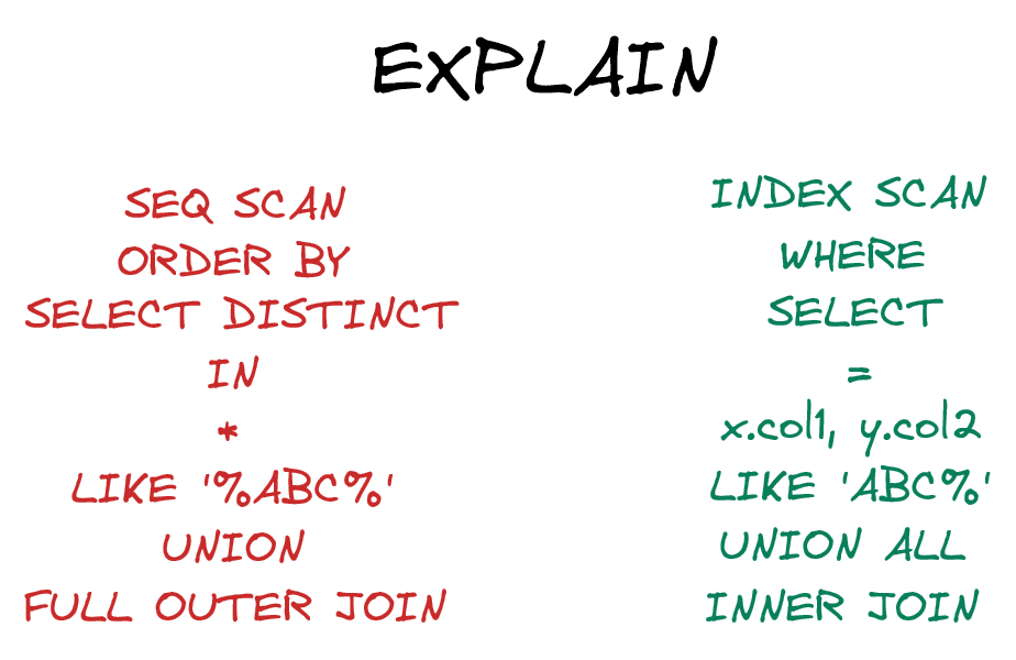
Looking under the hood: EXPLAIN
Let’s cover one final concept before closing out this post. The more knowledge we gain about SQL, the more ways we can build complex queries. Should we use EXCEPT or NOT IN? Should we perform a couple extra JOINs or use WITH and UNION ALL?
In essence, how do we know if one query is more or less efficient than another?
Postgres can actually tell you this. The keyword EXPLAIN provides an execution plan, which details how Postgres executes your query under the hood. Revisiting the query from the start of this post, we see that Postgres executes the query in a completely different order than how we wrote it.
| SQL |
1
2
3
4
5
6
7
8
9
10
11
12
13
14
15
16
17
18
19
20
21
22
23
24
25
26
EXPLAIN
SELECT
    s.id AS student_id,
    g.score
FROM
    students AS s
LEFT JOIN
    grades AS g
    ON s.id = g.student_id
WHERE
    g.score > 90
ORDER BY
    g.score DESC;

/*
 QUERY PLAN
 ----------
 Sort (cost=80.34..81.88 rows=617 width=8)
 [...] Sort Key: g.score DESC
 [...] -> Hash Join (cost=16.98..51.74 rows=617 width=8)
 [...] Hash Cond: (g.student_id = s.id)
 [...] -> Seq Scan on grades g (cost=0.00..33.13 rows=617 width=8)
 [...] Filter: (score > 90)
 [...] -> Hash (cost=13.10..13.10 rows=310 width=4)
 [...] -> Seq Scan on students s (cost=0.00..13.20 rows=320 width=4)
*/
We can take it a step further with EXPLAIN ANALYZE, which will run the query and detail the performance.
| SQL |
1
2
3
4
5
6
7
8
9
10
11
12
13
14
15
16
17
18
19
20
21
22
23
24
25
26
27
28
29
30
31
32
33
34
35
36
EXPLAIN ANALYZE
SELECT
    s.id AS student_id,
    g.score
FROM
    students AS s
LEFT JOIN
    grades AS g
    ON s.id = g.student_id
WHERE
    g.score > 90
ORDER BY
    g.score DESC;

/*
 QUERY PLAN
 ----------
 Sort (cost=80.34..81.88 rows=617 width=8)
   (actual tiem=0.169..0.171 rows=6 loops=1)
 [...] Sort Key: g.score DESC
 [...] Sort Method: quicksort Memory: 25kB
 [...] -> Hash Join (cost=16.98..51.74 rows=617 width=8)
   (actual time=0.115..0.145 rows=6 loops=1)
 [...] Hash Cond: (g.student_id = s.id)
 [...] -> Seq Scan on grades g (cost=0.00..33.13 rows=617 width=8)
   (actual time=0.045..0.052 rows=6 loops=1)
 [...] Filter: (score > 90)
   Rows removed by Filter: 19
 [...] -> Hash (cost=13.10..13.10 rows=310 width=4)
   (actual time=0.059..0.060 rows=5 loops=1)
 [...] Buckets: 1024 Batches: 1 Memory Usage: 9kB
 [...] -> Seq Scan on students s (cost=0.00..13.10 rows=310 width=4)
    (actual time=0.022..0.027 rows=5 loops=1)
 Planning Time: 0.379 ms
 Execution Time: 0.227 ms
*/
We see above, for example, that Postgres is sequentially scanning (Seq Scan) our grades and students tables because the tables aren’t indexed. In other words, Postgres has no idea whether rows later in the students table will have lower or higher IDs than earlier rows (if we were to index on ID). This suboptimal performance isn’t a huge concern for our tiny database, but if our database grew to millions of rows, we would definitely need to identify and fix bottlenecks such as these.[5]
Conclusions
This post was a broad overview of some SQL skills that become useful once you’re beyond the basics. We started by installing Postgres and pgAdmin, setting ourselves up for success by enabling experimentation with SQL on our own laptops.
We then covered useful syntax for building more elaborate queries. We started with filters, outlining the differences between WHERE and HAVING. We then discussed if-then logic, showing how to bucket values with CASE WHEN and handle nulls with COALESCE. We moved from horizontal to vertical merges with set operators, detailing how UNION, UNION ALL, INTERSECT, and EXCEPT keep some or all rows in the provided tables. We then ended this section by showing how to create and process arrays.
Next, we discussed components of more advanced queries, such as using self joins to join tables on themselves, window functions for comparisons within groups, and WITH to name subqueries. Finally, we discussed how EXPLAIN and EXPLAIN ANALYZE can quantify the performance of our queries and point to areas for improvement.
Want to keep expanding your knowledge? There are always more functions to learn, like CAST (for converting datatypes, e.g. floats to integers), or user-defined functions for simplifying your code further. These are useful, but I actually recommend thinking about optimizing your queries however possible. Even at FAANG companies with essentially unlimited compute, queries can fail if they demand more memory than a server can handle. Choosing the right approach for a complex query makes a data pipeline easier to maintain, meaning you’re less likely to get called at midnight when it breaks. (Hopefully!)
Best,
Matt

Footnotes
1. Setting up
What actually happens when we specify CASCADE when dropping a table? A little demo can be helpful.
Let’s say we drop classrooms without dropping any other tables. None of the data in students is affected – we still see the original classroom IDs.
| SQL |
1
2
3
4
5
6
7
8
9
10
11
12
13
14
15
16
17
18
19
20
21
22
23
24
25
26
27
28
29
30
31
32
33
34
35
36
37
38
SELECT
    s.name,
    s.classroom_id,
    c.teacher
FROM
    students AS s
LEFT JOIN
    classrooms AS c
    ON c.id = s.classroom_id;

/*
 name     | classroom_id | teacher
 -------- | ------------ | -------
 Adam     |            1 | Mary
 Betty    |            1 | Mary
 Caroline |            2 | Jonah
 Dina     |       [null] | [null]
 Evan     |       [null] | [null]
*/

DROP TABLE classrooms CASCADE;

/*
DROP TABLE
Query returned successfully in 71 msec.
*/

SELECT * FROM students;

/*
 id | name     | classroom_id | best_friend_id
 -- | -------- | ------------ | --------------
  1 | Adam     |            1 |              5
  2 | Betty    |            1 |              4
  3 | Caroline |            2 |              2
  4 | Dina     |       [null] |              2
  5 | Evan     |       [null] |              1
*/
If we now recreate classrooms and enter different teachers, the relation between students and classrooms is no longer accurate.
| SQL |
1
2
3
4
5
6
7
8
9
10
11
12
13
14
15
16
17
18
19
20
21
22
23
24
25
26
27
28
29
30
31
32
33
34
35
36
37
38
39
40
CREATE TABLE classrooms (
    id INT PRIMARY KEY GENERATED ALWAYS AS IDENTITY,
    teacher VARCHAR(100)
);

/*
CREATE TABLE
Query returned successfully in 139 msec.
*/

INSERT INTO classrooms
    (teacher)
VALUES
    ('Dr. Random'),
    ('Alien Banana');

/*
INSERT 0 2
Query returned successfully in 99 msec.
*/

SELECT
    s.name,
    s.classroom_id,
    c.teacher
FROM
    students AS s
LEFT JOIN
    classrooms AS c
    ON c.id = s.classroom_id;

/*
 name     | classroom_id | teacher
 -------- | ------------ | -----------
 Adam     |            1 | Dr. Random
 Betty    |            1 | Dr. Random
 Caroline |            2 | Alien Banana
 Dina     |       [null] | [null]
 Evan     |       [null] | [null]
*/
This is because CASCADE deleted the foreign key reference in students. We can see this by manually updating classroom_id in students (which is now not a foreign key) to an ID not in classrooms, but being unable to do so with student_id in grades (which is a foreign key).
| SQL |
1
2
3
4
5
6
7
8
9
10
11
12
13
14
15
16
17
18
19
UPDATE students
SET classroom_id = 10
WHERE id = 1;

/*
UPDATE 1
Query returned successfully in 37 msec.
*/

UPDATE grades
SET student_id = 10
WHERE id = 1;
/*
ERROR:  insert or update on table "grades" violates foreign key
    constraint "fk_students"
DETAIL:  Key (student_id)=(10) is not present in table
    "students".
SQL state: 23503
*/
One final note on CASCADE. If we specify ON DELETE CASCADE when creating the foreign key in students, then deleting rows in classrooms will delete the linked rows in students. This can be important for privacy reasons, for example, if you want to delete all information about a customer or employee once they leave your company.
| SQL |
1
2
3
4
5
6
7
8
9
10
11
12
13
14
15
16
17
18
19
20
21
22
23
24
25
26
27
28
29
30
31
32
33
34
35
36
DROP TABLE IF EXISTS students CASCADE;

CREATE TABLE students (
    id INT PRIMARY KEY GENERATED ALWAYS AS IDENTITY,
    name VARCHAR(100),
    classroom_id INT,
    CONSTRAINT fk_classrooms
        FOREIGN KEY(classroom_id)
        REFERENCES classrooms(id) ON DELETE CASCADE
);

INSERT INTO students
    (name, classroom_id)
 VALUES
    ('Adam', 1),
    ('Betty', 1),
    ('Caroline', 2);

SELECT * FROM students;
/*
 id | name     | classroom_id
 -- | -------- | ------------
  1 | Adam     |            1
  2 | Betty    |            1
  3 | Caroline |            2
*/

DELETE FROM classrooms
WHERE id = 1;

SELECT * FROM students;
/*
 id | name     | classroom_id
 -- | -------- | ------------
  3 | Caroline |            2
*/
2. Setting up
Codifying our database schema is an engineering best practice, but for the actual data, we’ll instead perform database backups. There’s a variety of ways to do this ranging from memory-heavy full backups to relatively light snapshots of changes. Ideally, these files are sent somewhere geographically distant from the servers storing our database, so a natural disaster doesn’t wipe out your entire company.
3. Setting up
We specified the teacher column as a string with a max of 100 characters since we don’t think we’ll run into names longer than this. But are we actually saving on storage space if we limit rows to 100 characters versus 200 or 500?
In Postgres it turns out it technically doesn’t matter whether we specify 10, 100, or 500. So specifying a limit might be more of a best practice for communicating to future engineers (including yourself) what your expectations are for the data in this column.
But in MySQL the size limit does matter: temporary tables and MEMORY tables will store strings of equal length padded out to the maximum specified in the table schema, meaning a VARCHAR(1000) will waste a lot of space if none of the values approach that limit.
4. If-then: CASE WHEN & COALESCE
If you’re curious, here’s what Postgres code with an IF statement looks like.
| SQL |
1
2
3
4
5
6
7
8
9
10
11
12
13
14
15
16
17
DO $$

BEGIN
    IF
        (SELECT COUNT(*) FROM grades) >
        (SELECT COUNT(*) FROM students)
    THEN
        RAISE NOTICE 'More grades than students.';
    ELSE
        RAISE NOTICE 'Equal or more students than grades.';
    END IF;

END $$;

/*
NOTICE: More grades than students.
*/
5. Looking under the hood: EXPLAIN
Setting indexes on your tables is critical to ensuring performance as the database size grows. We can easily set an index on the scores in grades, for example, with the following query:
| SQL |
1
2
3
4
CREATE INDEX
    score_index
ON
    grades(score);
Yet, if we run EXPLAIN ANALYZE again, we’ll see that Postgres still runs a sequential scan. This is because Postgres has been optimized beyond what an “intermediate SQL” blog post will teach you! If the number of rows in a table are relatively small, it’s actually faster to perform a sequential scan than use an index, so Postgres executes the query with the faster approach.