
Learning R 5. The apply functions
#r
Written by Matt Sosna on February 1, 2017
Learning R series
- Introduction
- Random data and plotting
forloops and random walks- Functions and
ifstatements - The
applyfunctions
We’ve reached the point in learning R where we can now afford to focus on efficiency over “whatever works.” A prime example of this is the apply functions, which are powerful tools to quickly analyze data. The functions can find slices of data frames, matrices, or lists and rapidly perform calculations on them. These functions make it simple to perform analyses like finding the variance of all rows of a matrix, or calculating the mean of all individuals that meet conditions X, Y, and Z in your data, or to feed each element of a vector into a complex equation. With these functions in hand, you will have the tools to move beyond introductory knowledge of R and into more advanced analyses.
This is the fifth in a series of posts on R. This post covers:
apply,sapply,tapply,lapply(pronounced “apply,” “s-apply,” “t-apply,” and “l-apply”)sweep
The most important code from previous posts is shown below:
| R |
1
2
3
4
5
6
7
8
9
10
11
12
13
14
15
16
17
18
19
20
21
22
23
24
25
26
27
c()             # Concatenate
x <- c(5, 10)   # x is now a two-element vector
x[x > 7]        # Subset the values of x that are greater than 7

# Assign to the object "data" 100 randomly-drawn values from a normal
# distribution with mean zero and standard deviation 1
data <- rnorm(100)

# Plot a histogram of the "data" object
hist(data)

# Assign to the object "y" 100 randomly-drawn values from a uniform
# distribution with minimum zero and maximum 1
y <- runif(100)

# Make a scatterplot of y as a function of data
plot(y ~ data)

for(i in 1:length(x)){    # For i in the sequence 1 to the length of x...
   print(i)               # ...print i
}

# Create our own mean function
our.mean <- function(x){sum(x) / length(x)}

# Print the statement "Yup, less than 5" if 1 + 1 < 5 is true
if(1 + 1 < 5){print("Yup, less than 5")}
apply
The first of the apply functions is the one the family is named after. Let’s revisit the following plot from the third R post on for loops.
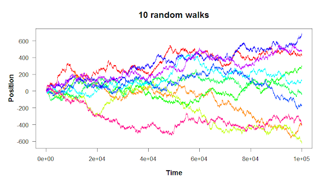
A random walk, if you remember, is a series of random steps. The walk can be in as many dimensions as you want; the ten walks shown above are in one dimension (where there’s only one movement axis: up/down). It seems like the variance in the walks increases with time: the more you move to the right, the more spread out the walks are. How could we quantify this?
In case you missed it, here’s how we generated the data for the above figure. But this time, let’s run 100 random walks instead of 10.
| R |
1
2
3
4
5
6
7
8
9
10
11
12
13
14
15
16
17
start <- 0
mean.step <- 0
sd.step <- 1
n.steps <- 100000
n.walks <- 100             # The number of random walks you want to run

# Create an empty matrix that we'll fill with the random walk values
WALKS <- matrix(NA, nrow = n.walks, ncol = n.steps)

# Start all the walks at the origin
WALKS[, 1] <- start

# Perform the random walks
for(i in 2:n.steps){
    WALKS[, i] <- WALKS[, i-1] +        # Take the previous positions...
    rnorm(n.walks, mean.step, sd.step)  # ...and add a step to each one
}
[Note: if you did rnorm(1, ...), you would generate 100 identical random walks because the same value would be added to each walk. That’s why we need to specify the number of random walks in the first argument in rnorm.]
WALKS is a 100 x 100,000 matrix, where each row is a random walk and each column is a time point. To show how the variance of the walks changes over time, we want to take the variance of each column. One way to do this would be to create a for loop that iterates over each column:
| R |
1
2
3
4
5
walk.variance <- c()
for(i in 1:ncol(WALKS)){
   walk.variance[i] <- var(WALKS[, i])
   print(i)
}
This works, but there’s a simpler way to do this. Let’s use apply, which only requires one line of code.
| R |
1
walk.variance <- apply(WALKS, 2, var)
apply’s inputs are the matrix, whether you want rows (apply(..., 1, ...)) or columns (apply(..., 2, ...)), and the function you want to apply to that dimension of the matrix, which for us is var.
[Note: you can also do this for higher-dimensional arrays, e.g. a 3-dimensional “book” where you want to summarize each “page.” That would be apply(..., 3, ...)]
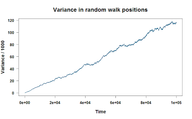
If we plot walk.variance, we see a nice linear relationship between the variance and how long we’ve run the random walk.
You can apply any function to each column or row, as long as it can take a vector input. Using what we learned in post 4 of our R series, let’s apply a more complicated function to each row of the matrix. This function will find the mean of the six highest values of each random walk, then subtract it from the range. No real reason why. Just flexing a little R muscle!
| R |
1
2
3
4
5
6
7
# Find the mean of the six highest values of the input,
# then subtract it from the range
fun.times <- function(x){
    return(mean(head(x)) - (range(x)[2] - range(x)[1]))
}

lots.of.fun <- apply(WALKS, 1, fun.times)
sweep
apply is great for performing a calculation on each row or column of a matrix, but what if you want to, say, subtract an entire vector across each column of a matrix? You’re not subtracting just one value from the matrix. You have a separate value for each column. For this, you’ll want sweep.
Here’s a simple example that doesn’t require sweep. You’re subtracting one value from the entire matrix.
| R |
1
WALKS.adjusted <- WALKS - mean(WALKS)
Here, the new object (WALKS.adjusted) has been centered around the mean of WALKS. This isn’t incredibly informative, though, because the mean of WALKS condenses the information from all the random walks and all the time points of those walks into one value.
With sweep, we can be more nuanced. Let’s create a new matrix, WALKS.adjusted2, where all of the walks are centered around the mean of all the random walks for that particular time point. Walks that are have particularly high values will have positive values, average walks will be around zero, and walks with low values will have negative values.
| R |
1
WALKS.adjusted2 <- sweep(WALKS, 2, colMeans(WALKS), "-")
In English, the code above says subtract ("-") the mean of each column (colMeans(WALKS)) from each column (2) of WALKS.
sapply
apply works great on matrices, but it doesn’t work if you want to perform a calculation on every element of a vector, or if you want to perform a calculation on only select columns of a matrix or data frame. In these cases, sapply is the answer. sapply takes in a vector, matrix, or list (a data type we’ll cover here) and returns a vector. In this post, we’ll just focus on using sapply on vectors[1].
Let’s say we have a list of probabilities, and we want to simulate outcomes based on those probabilities. Maybe we have 50 friends, each with some probability of wanting to marathon the eight Harry Potter movies back to back in a massive sleepover party. We can simulate “rolling the dice” on a vector of those probabilities with sapply.[2].
| R |
1
2
3
4
5
6
7
8
9
10
11
12
13
14
15
16
17
# 50 random values drawn from a uniform distribution between 0 and 1
probs <- runif(50, 0, 1)

# The possible outcomes
outcomes <- c("It's marathon time!",
              "Sorry, I actually already have plans...")

# A function that returns an outcome, given a probability
prob_to_outcome <- function(x){sample(outcomes, 1, prob = c(x, 1-x))}

result <- sapply(probs, FUN = prob_to_outcome)

print(result)
# > "Sorry, I actually already have plans..."
#   "Sorry, I actually already have plans..."
#   "It's marathon time!"
#   ...
prob_to_outcome takes in a probability of wanting to marathon the Harry Potter movies and simulates whether the person ended up choosing to marathon the series or not. In line 11, sapply runs prob_to_outcome on every probability in probs. We could do the same with a for loop, but it would be both more lines of code and less efficient:
| R |
1
2
3
4
5
# Less efficient version of line 11 above
result <- c()
for(i in 1:length(probs)){
    result[i] <- prob_to_outcome(probs[i])
}
tapply
While you can use sapply on data frames[1], tapply is a friendlier tool. Let’s say we successfully hosted our Harry Potter marathon and we surveyed our guests on how they rank the eight films. Our data is vertically stacked in a dataframe like this. And for a bit of fun, we also know whether they consider themselves Twilight fans or not.
We’ll start by defining some variables:
| R |
1
2
3
4
5
6
7
n_movies <- 8
n_guests <- 10

titles <- c("Sorcerer's Stone", "Chamber of Secrets",
            "Prisoner of Azkaban", "Goblet of Fire",
            "Order of the Phoenix", "Half-Blood Prince",
            "Deathly Hallows p.1", "Deathly Hallows p.2")
Then we’ll loop through our guests, generate a dataframe with each guest’s info, and stacking the dataframes on top of one another. We could avoid using a for loop here, but given the fact that we’re vertically stacking data and dealing with both single values (guest_id, being a fan of Twilight) and vectors (titles, rankings), it’s a lot clearer to use a loop.
| R |
1
2
3
4
5
6
7
8
9
10
11
12
13
14
15
16
17
for(i in 1:n_guests){

    rankings <- sample(1:n_movies, n_movies, replace=F)
    twilight_fan <- sample(c(TRUE, FALSE), 1)

    df_guest <- data.frame('guest_id' = i,
                           'twilight_fan' = twilight_fan,
                           'movie' = titles,
                           'rank' = rankings)

    # Start df_final or add to it
    if(i == 1){
        df_final <- df_guest
    } else {
        df_final <- rbind(df_final, df_guest)
    }
}
Now we can actually analyze our data. Let’s ask what the average rank is for each movie. With tapply, the first argument is the data to analyze, the second argument is how to group the data, and the third is the function to apply.
| R |
1
2
3
4
5
6
7
tapply(df$rank, df$movie, mean)
#   Chamber of Secrets   Deathly Hallows p.2   Deathly Hallows p.1
#                  4.2                   4.0                   5.2
#       Goblet of Fire     Half-Blood Prince  Order of the Phoenix
#                  3.4                   4.3                   4.7
#  Prisoner of Azkaban      Sorcerer's Stone
#                  5.0                   5.2
Looks like Goblet of Fire wins! (Let’s just ignore any semblance of statistical rigor.) But what about for people who like vs. dislike Twilight? For this extra nuance, we can just modify the second argument in tapply to include both df$movie and df$twilight_fan. As a step further to keep the code clean, I’ll use the with command, which lets us avoid needing to type df$ before any column in df.
| R |
1
2
3
4
5
6
7
8
9
10
with(df, tapply(rank, list(movie, twilight_fan), mean))
#                       FALSE TRUE
#  Chamber of Secrets     2.0 4.75
#  Deathly Hallows p.2    3.0 4.25
#  Deathly Hallows p.1    6.0 5.00
#  Goblet of Fire         6.0 2.75
#  Half-Blood Prince      6.5 3.75
#  Order of the Phoenix   3.5 5.00
#  Prisoner of Azkaban    2.0 5.75
#  Sorcerer's Stone       7.0 4.75
In a shocking upset, turns out the best-ranked film is a tie between Chamber of Secrets and Prisoner of Azkaban for people who don’t like Twilight. For those who do like Twilight, Goblet of Fire reigns again. But to see if any of these insights are worth making it past a toy example in a blog post, we’ll want a much bigger representative sample of… real people.
lapply
Finally, we have lapply, a function that lets you apply a function to every element of a list. In R, lists are objects that contain other objects. We can create a sample list, L, that has the numbers 1 to 3, a string, and a dataframe.
| R |
1
2
3
4
5
6
7
8
9
10
11
L <- list(1:3, 'hello', data.frame('id'=1))
L
# [[1]]
# [1] 1 2 3
#
# [[2]]
# [1] "hello"
#
# [[3]]
#    id
#  1  1
With lapply, we can efficiently apply a function to each object in the list. It doesn’t make a whole lot of sense, but we could, for example, apply min to each element. Note that lapply returns a list[3].
| R |
1
2
3
4
5
6
7
8
9
lapply(L, min)
# [[1]]
# [1] 1
#
# [[2]]
# [1] "hello"
#
# [[3]]
# [1] 1
Let’s finish this post with an example that is more sensible and has more Harry Potter in it. In an effort to get on the front page of /r/dataisbeautiful, we decide to collect some data at our party. Every 30 minutes, we poll the audience on how much fun they’re having. (It’d be solid 10/10’s throughout the night, but play along and imagine there’s some variation.) With these data, we build a matrix where each row is a party participant and each column is a time point (3:10am, 3:20am, etc.). The data are how much fun person i is having at time point j.
| R |
1
2
3
4
5
6
7
8
9
10
11
12
13
14
15
n_samples <- 100
n_guests <- 10

fun_mat <- matrix(round(runif(5000, 0, 10)),
                  ncol = n_samples, nrow = n_guests)
rownames(fun_mat) <- sapply(1:nrow(fun_mat), function(x){paste0("person", x)})
colnames(fun_mat) <- sapply(1:ncol(fun_mat), function(x){paste0("t", x)})

print(fun_mat)
#          t1 t2 t3 t4 t5 t6 t7 t8 t9 t10 t11 t12 t13 t14 ...
# person1   7  7  5  7  5  1  1  7  7   5   0   7   8   9 ...
# person2   6  9  5 10  4  2  2  1  2   9   0   1   1   5 ...
# person3   8  1  7  4  5  1  3  5  4   1   8   9  10   1 ...
# person4   2  1  2 10  1  2  8  5  1   6   6   5   0   0 ...
# ...
What if we want to know what moments each person was having at least 9/10 fun? We could just write which(fun_mat >= 9), but that would convert fun_mat into a vector and then return the indices of the vector where the value is greater than 9. So for our 100 x 50 matrix, we’d get answers like 9 and 738 and 2111, which don’t have any identifying information on who was happy when.
This sounds like a job for apply, so we run this:
| R |
1
2
3
4
5
6
7
8
9
10
passed_threshold <- apply(fun_mat, 1, function(x){which(x >= 9)})
print(passed_threshold)
# $person1
#     t2  t6  t23  t27  t53  t76
#      2   6   23   27   53   76
#
# $person2
#     t1  t2  t30  t32  t40  t47  t48  t50  ...
#      1   2   30   32   40   47   48   50  ...
# ...
We now have a list, where each object is a person, and the values are the time points at which they scored at least a 9/10 on having fun. However, we can now use lapply to get more nuanced information from passed_threshold. Here is the first time point at which someone passed the threshold of having fun:
| R |
1
2
3
4
5
6
7
8
# Find the first time point that passed the threshold
lapply(passed_threshold, min)
# $person1
# [1] 2
#
# $person2
# [1] 1
# ...
And here is a full summary of when having fun occurred:
| R |
1
2
3
4
5
6
7
8
9
10
# Get a summary of the time points for each person that
# passed the threshold
lapply(passed_threshold, summary)
# $person1
#    Min. 1st Qu.  Median    Mean 3rd Qu.    Max.
#    2.00   10.25   25.00   31.17   46.50   76.00
#
# $person2
#    Min. 1st Qu.  Median    Mean 3rd Qu.    Max.
#    1.00   36.00   50.00   51.87   76.50   90.00
Note that these commands return their contents as a list. If you’d prefer they were returned as a vector, we can use sapply instead.
| R |
1
2
3
sapply(passed_threshold, min)
# person1  person2  person3  person4  person5  person6  ...
#       2        1        4        3        6        9
Conclusions
Thanks for reading the “Introduction to R” series! If you want to keep learning R, check out some “Random R” posts in the blog page. You can find little experiments in there like racing for loops vs. apply, visualizing GPS data, and more.
Cheers,
-Matt
Footnotes
1. sapply
We can also use sapply on dataframes and matrices when we only want to run our calculation on specific columns. Let’s say we run a lab experiment and have the results in a dataframe that has columns for our data, as well as metadata like the date of the trial, the treatment name, etc. If we want to find the median of our data columns, we can’t just do apply - R will complain about trying to find the median for the non-numeric columns. Instead, we can get the indices of the numerical columns and then use sapply.
| R |
1
2
3
4
5
6
7
8
9
10
11
12
# Generate sample data
height_gain <- rnorm(20)
weight_gain <- rnorm(20)
treatment <- sort(rep(c("medicine", "placebo"), 10))
trial <- factor(rep(1:5, 4))   # Indicate vals are factors, not ints

df <- data.frame(height_gain, weight_gain, treatment, trial)

numeric_cols <- sapply(df, is.numeric)
sapply(which(numeric_cols), function(x){median(df[, x])})
# > height_gain weight_gain
#   2.683714    -2.070083
You’ll notice we call sapply twice - first to get a vector of booleans (TRUE and FALSE) for whether each column in df is numeric, and then again to find the median of each numeric column. [Because numeric_cols is a vector of TRUE and FALSE values, we don’t have to specify which(numeric_cols == T); which already only returns indices that are TRUE.]
However, while it’s possible to use sapply like this, I find it more convenient to use tapply so we can avoid using indices (and can instead use column names, which is easier to verify that we’re doing what we think we’re doing). We can even get away with using apply again, such as with apply(df[, which(numeric_cols)], 2, median). So I usually stick with analyzing vectors with sapply, which is why this section is a footnote instead of in the main text.
2. sapply
Note that when we simulate outcomes based on probabilities, the outcomes will differ between runs - if we have a probability of 0.5, for example, we can expect roughly half our runs to have a positive outcome and half to have a negative. If you want to control this randomness (e.g. for sharing a reproducible analysis), use set.seed to force the next random function to always return the same value.
| R |
1
2
3
4
5
6
7
8
9
10
# Without seed
rnorm(3)  # 1.2724293  0.4146414 -1.5399500
rnorm(3)  # -1.1476570 -0.2894616 -0.2992151

# With seed
set.seed(1)
rnorm(3)  # -0.6264538  0.1836433 -0.8356286

set.seed(1)
rnorm(3)  # -0.6264538  0.1836433 -0.8356286
3. lapply
We can actually run sapply on the list to get our result as a vector, though the response might seem confusing.
| R |
1
sapply(L, min)   # "1"  "hello"  "1"
Why are the first and third elements strings instead of integers? This is because vectors in R must have elements of the same type. Because we have both integers and strings when we apply min to each element of L, R needs to choose one of the two data types for our vector. The number 1 has a clear conversion to the string "1", but there’s no obvious integer to convert "hello" to. R therefore converts all elements to strings before returning the vector.