Learning R
3. For loops and random walks

#r
Written by Matt Sosna on April 24, 2016

Learning R series

When I was a teenager, I didn’t mind repetitive, mindless labor. To document my musical tastes, every few months I’d gather data from my iTunes library, manually counting the number of songs that I had listened to 0, 1, 2, 3, up to 6 times so I could create a histogram in Excel. I loved office work like stapling papers for hours, and pipetting was one of my favorite aspects of the evolutionary development lab I briefly worked in during college. (Side note: my favorite aspect was feeding the opossums, which made me realize I loved animal behavior.)

Well, times change. At some point, you just can’t resort to human willpower to get through an analysis. Fortunately, computers are fantastic for work that would otherwise be menial and soul-draining. They don’t get bored as far as we can tell, they’re much faster, and they don’t make mistakes if the code is correct.

This is the second post in a series on R. This post covers:

for loops
Random walks

The first post was an introduction to R, and the second was on using R to understand distributions, plotting, and linear regression. The most important code from those posts is listed below.

# "Concatenate." This is how you create vectors in R
c()  

# Assign to x a two-element vector of the numbers 5 and 10
x <- c(5, 10)

# Subset x on only the values greater than 7
x[x > 7]

# Draw 100 random values from a normal distribution with mean = 0
# and standard deviation = 1
data <- rnorm(100)  

# Plot a histogram of the data object
hist(data)

# Plot a scatterplot of y as a function of x
plot(y ~ x)  

`for` loops

for loops are basically a way to iterate, or to run a command repeatedly. (Think of the word “reiterate,” for example: “I had to reiterate to my cat to not use my Gmail without permission. It’s the third time this week. I just don’t think he’s old enough to use the internet unsupervised.”)

Here’s a super simple for loop:

for(i in 1:10){
  print(i)
}

It reads “for i in the sequence 1 to 10, print i.” It’s the same as if you wrote this:

print(1)
print(2)
print(3)
print(4)
print(5)
print(6)
print(7)
print(8)
print(9)
print(10)

A for loop finds wherever you placed an i within the loop and changes that to the i-th value in the sequence you give it (here it’s 1:10). The first value in the sequence above is 1, the second is 2, etc.

The sequence you give the for loop doesn’t have to be linear. You could write whatever bunch of numbers you want. Writing this…

bubbles <- c(1, -80, 4, NA, 100, -Inf, 0)
for(bub in bubbles){
    print(bub)
}

… is the same as writing this:

print(1)
print(-80)
print(4)
print(NA)
print(100)
print(-Inf)
print(0)

You’ll also get the same thing if you tell R that you want the ith value of bubbles. This is a subtle distinction. Instead of iterating through the actual values in bubbles, the for loop will iterate through the 1st value, then the 2nd, then the 3rd, until it reaches the end. Iterating through an index is often a nicer way to structure your loop^[1].

for(i in 1:length(bubbles)){  # "For i in 1 to the length of 'bubbles'...
    print(bubbles[i])         # ...print the ith value of bubbles."
}

The above code is the same thing as writing:

print(bubbles[1])
print(bubbles[2])
print(bubbles[3])
print(bubbles[4])
print(bubbles[5])
print(bubbles[6])
print(bubbles[7])

Combine `for` loops with `paste` for strings

All of the values in bubbles above are numbers, which makes things simple. It’s only slightly more challenging if you have a bunch of words, or you’re trying to iterate a sentence.

Let’s say you want to type out "Today is April 1," "Today is April 2," "Today is April 3,", all the way up to "Today is April 30." Maybe you really love April or something. In R, you could literally write:

print("Today is April 1")
print("Today is April 2")
print("Today is April 3")
print("Today is April 4")

… and so on. That would be 30 lines of code. Manageable, but not great. Alternatively, you could use a for loop combined with the paste command.

for(i in 1:30){
  print(paste("Today is April", i))
}

If you wrote print("Today is April i"), it will say “Today is April i” instead of replacing the i with whatever number you’re on. paste lets you input values into character strings. For example:

names <- c("Matt", "George", "Andre")
for(i in 1:length(names)){
 paste("My name is", names[i])
}   

Real world example

In my Ph.D., I work with animal tracking data. I’ll film experiments involving fish swimming in a tank. These videos then get fed through tracking software that identifies the positions and orientations of all individuals. These data are in the form of four matrices: the x- and y-coordinates for each fish for each frame, as well as the x- and y-components of the unit vector of their heading. Each row of a matrix is one individual, and each column is a time point.

From these simple matrices, I can calculate more interesting measurements like the speed and distance to nearest neighbor for every fish. Below is the code for calculating the speed time series for each individual.

First, we create an empty matrix, sp, with the same dimensions as the xs matrix (our matrix of x-coordinates). We could also use the ys matrix - all that matters is that the dimensions are the number of fish for rows, and number of columns

sp <- matrix(NA, ncol = ncol(xs), nrow = nrow(xs))

We then calculate how far a fish moved between time points. We’ll iterate over each fish.

# Iterate through the rows of sp
for(i in 1:nrow(sp)){           

    # This row of sp gets assigned a vector where the first value is
    # NA (because speed is a *difference* of two positions)...
    sp[i, ] <-  c(NA,     

        # ...and the rest of the vector is the Pythagorean theorem on
        # the corresponding rows in the x- and y-position matrices
        sqrt(diff(xs[i, ])^2 + diff(ys[i, ])^2)
    )  

    # Print the iteration we're on
    print(i)
}

If we wanted to plot one of the individual’s trajectories from time point 1000 to 2000, we could do so like this:

# Plot Individual 6's trajectory from time point 1000 to 2000
focal_indiv <- 6
time_start <- 1000
time_end <- 2000

plot(sp[focal_indiv, time_start:time_end],
     main = paste("Individual", focal_indiv, "speed from t =",
                  time_start, "to t =", time_end)

Random walks

for loops are ideal for when you need to iterate a computation. A simple example of this is a random walk, which is a series of random steps. It’s a time series that serves as a null expectation: “what should we expect to see if literally nothing but noise is happening?” It’s a baseline that you can then compare to stock market prices, animal movement, gas molecule paths, and more.

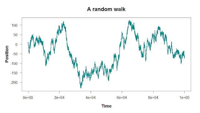
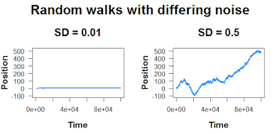
Here, these peaks and valleys aren’t caused by any extrinsic factor; they’re just random fluctuations. The size of these fluctuations will depend on how much noise you add into the random walk:

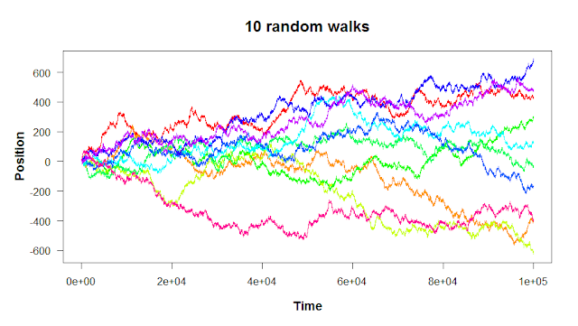
And finally, remember that “random” means it’s not going to be the same every time.

There are two steps to building a random walk in R: first, you set the starting point and the rules for the steps. Then, you run a for loop to take each step. Let’s walk through the code to build a simple one-dimensional random walk like the plots above.

First, we set the parameters of the walk. We’ll want the starting point for each walk - zero is usually a good place to start (start <- 0). Then, we’ll want to set the parameters of the distribution from which we draw our random steps. We’ll use a normal distribution, which is straightforward to understand. Our normal distribution will be centered at zero (mean_step <- 0)^[2] with a standard deviation of 1 (sd_step <- 1). This means that most of our steps will be close to zero, with values further from zero occurring less frequently. If we wanted a wider-ranging walk, we could crank up sd_step to a higher number.

# Parameters
start <- 0          # The starting point of the random walk
mean_step <- 0      # The walk bias
sd_step <- 1        # The standard deviation of the step size
n_steps <- 100000   # The number of steps to take

With our parameters set, now we can actually generate the walk. We start by setting our random walk, which we’ll just call walk, equal to our starting location (start). Then, we iterate from 2:n_steps, calculating the next location in the walk by 1) taking the previous location and then 2) taking a step generated from our distribution. Finally, we print i for each iteration to see if our code is getting stuck anywhere or running slower than we think it should.

# Begin the walk at the starting point
walk <- start

# Run the random walk
for(i in 2:n_steps){   # Start at 2 because we already have our  
                       # starting point
   walk[i] <- walk[i - 1] +         # Take the previous position...
      rnorm(1, mean_step, sd_step)  # ... and add a random value
   print(i)                         # Tell us what iteration we're on
}

Finally, to visualize our results, we can use the plot command: plot(walk, type = 'l'). Done!

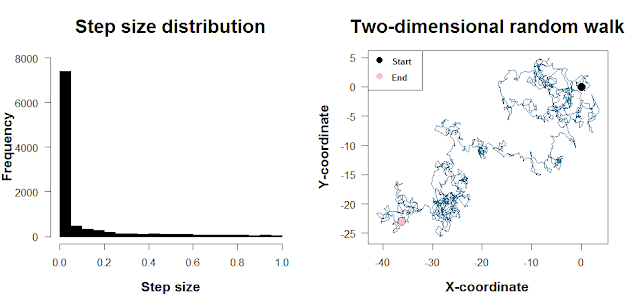
In the above walk, we use a normal distribution as the source of our step sizes. It means that most of our steps will be concentrated around mean_step, with large step sizes (in either direction) occurring less frequently. The normal distribution is convenient, but in R it’s just as convenient to use a different distribution like a long-tailed distribution (e.g. for a Lévy flight) or a Poisson. The plot below shows such a skewed step size distribution and what a two-dimensional random walk with steps drawn from this distribution looks like. The code to do this is at the end of this post. [There’s a bit more to mention with the direction of travel as well as the step sizes, but I’ll skip the details here.]

Wait, should I use `for` loops?

The short answer is yes… as long as they’re written well!

The first thing you learn about for loops is what they are. The second thing you learn about for loops is that it’s really easy to write them in a way that’s computationally inefficient. While computers are very good at calculating many things simultaneously, for loops force R to focus on one thing at a time. This is usually not a big deal: for small computations like the ones listed in this post, we rarely encounter a situation where for loops won’t work well. And if we avoid mistakes with how we update our variables, for loops are often fine.

# Pull files to extract info from
bunch_of_files <- list.files()

overall_results <- c()

for(i in 1:length(bunch_of_files)){

    file_result <- function_that_takes_forever(files[i])

    # DON'T do this:
    overall_results <- c(overall_results, file_result)

    # DO this instead:
    overall_results[i] <- file_result
}

Especially when it comes to mathematical operations, there are often vectorized approaches that let you run many calculations in parallel instead of forcing R to do them one by one with a for loop. For example, we can actually calculate our speed matrix from earlier without iterating through each row.

# With a for loop
sp <- matrix(NA, ncol=ncol(xs), nrow=nrow(xs))

for(i in 1:nrow(sp)){
    sp[i, ] <- c(NA, sqrt(diff(xs[i, ])^2 + diff(ys[i, ])^2))
}

# Without a for loop
sp <- cbind(NA, sqrt(t(diff(t(xs)))^2 + t(diff(t(ys)))^2))

If we have a millions or billions of calculations to compute, the single-track nature of for loops can quickly become impractical. Imagine a model that simulates how predator-prey population dynamics evolve under various levels of resource availability. R will need to calculate all predator-prey interactions for a generation, for every generation, for every run of the model… for every combination of parameter values. Without exaggerating, your model could literally require years of computational time to complete if you’re chugging away with one for loop.

If you find yourself in that situation (and are determined to stay in R), you’ll likely need to delve into R packages that let you simultaneously run code in parallel, which taps into your computer’s ability to have multiple processes running at once. If you’re even more hardcore, you’ll want to look into packages that optimize C++ code, which R runs under the hood.

Cheers,
-Matt

Footnotes

1. For loops

When you iterate through an index instead of the values themselves, you can more easily update other variables with the results of the loop.

result_vec <- c()
for(i in 1:length(input_vec)){
    result_vec[i] <- some_function(values[i])
}

(In this specific example, I’d actually look for a way to vectorize some_function so you can process all values in input_vec at once, e.g. result_vec <- vectorized_func(values). But you get the point!)

2. Random walks

Note that we could set mean_step equal to some positive or negative value; that just means that our walk would drift upward or downward. By setting it to zero, our walk is unbiased: at each iteration, it’s equally likely to take a step downward as it is to take a step upward.

Code for plots

First random walk

start <- 0            # Starting position
mean_step <- 0        # The step distribution will be unbiased
sd_step <- 1          # The standard deviation of step sizes
n_steps <- 100000     # The number of steps

walk <- start         # Start the walk at the origin

for(i in 2:n_steps){

    # This step is the previous step plus...
    walk[i] <- walk[i - 1] +

        #... a random value from our distribution of steps     
        rnorm(1, mean_step, sd_step)  

}

plot(walk, type = 'l', col = "darkcyan", lwd = 2,
     xlab = "Time", ylab = "Position", las = 1,
     main = "A random walk", cex.main = 1.5, cex.lab = 1.2, font.lab = 2)

Random walks with differing noise

start <- 0
n.steps <- 1e5

mean.step <- 0
sd.step1 <- 0.01
sd.step2 <- 0.5

# Start both walks at zero
walk1 <- walk2 <- start

for(i in 2:n.steps){
  walk1[i] <- walk1[i - 1] + rnorm(1, mean.step, sd.step1)
  walk2[i] <- walk2[i - 1] + rnorm(1, mean.step, sd.step2)
  print(i)
}

# Plot it
par(mfrow = c(1,2))    # Split into two subplots
par(oma = c(0,0,2,0))  # Create space at the top for a grand title

plot(walk1, type = 'l', col = "dodgerblue",
     main = paste("SD =", sd.step1), font.lab = 2,
     xlab = "Time", ylab = "Position", ylim = c(min(walk2), max(walk2)))
plot(walk2, type = 'l', col = "dodgerblue",
     main = paste("SD =", sd.step2), font.lab = 2, xlab = "Time",
     ylab = "Position", ylim = c(min(walk2), max(walk2)))
mtext(outer = T, "Random walks with differing noise", cex = 2, font = 2)

par(oma = array(0, 4)) # Make your graphics window look normal again

Multiple random walks

start <- 0
mean.move <- 0
sd.move <- 1
n.steps <- 100000
n.indivs <- 10             # The number of random walks you want to run

# Create an empty matrix that we'll fill with the random walk values
WALK <- matrix(NA, nrow = n.indivs, ncol = n.steps)

# Start all the walks at the origin
WALK[, 1] <- start

# Perform the random walks
for(i in 2:n.steps){

    # Start at the previous time step's values
    WALK[, i] <- WALK[, i - 1] +         

        # Generate 10 random values, one for each row (if you did
        # rnorm(1, ...), you'd generate 10 identical walks because
        # the same value would be added to each walk
        rnorm(n.indivs, mean.move, sd.move)  

    print(i)
}

# First create an empty plot, then add each walk with a for loop
plot(NA, ylim = c(min(WALK), max(WALK)), xlim = c(0, n.steps),
     cex.main = 1.5, cex.lab = 1.2, xlab = "Time", ylab = "Position",
     las = 1, font.lab = 2, main = "10 random walks")

for(i in 1:nrow(WALK)){
 lines(WALK[i,], col = rainbow(n.indivs)[i])
}

Two-dimensional random walk

# Use a highly skewed beta distribution for the step sizes
# - Very likely to take small step, unlikely to take big step
step.dist <- rbeta(10000, 0.1, 1)

# Set the parameters for the (Gaussian) turning angle distribution
mean.turn <- 0
sd.turn <- pi/4

# Starting positions and orientations
# - Orientation could start at zero; here it's random
xs <- ys <- 0
BO <- runif(1, -pi, pi)

# Run it
for(i in 2:t){   
   # Update the heading and step size
   BO[i] <- BO[i - 1] + rnorm(1, mean.turn, sd.turn)
  step.size <- sample(step.dist, 1)

  # Take steps
  # cosine gives x-component of unit vector, sine gives y-component
  xs[i] <- xs[i - 1] + cos(BO[i]) * step.size   
  ys[i] <- ys[i - 1] + sin(BO[i]) * step.size   

  print(i)
}

Written on April 24, 2016

Learning R 3. For loops and random walks

for loops

Combine for loops with paste for strings