
Learning R 1. Introduction
#r
Written by Matt Sosna on December 15, 2015
Learning R series
- Introduction
- Random data and plotting
forloops and random walks- Functions and
ifstatements - The
applyfunctions
When I first encountered R in 2011, I was a junior in college. I had heard about it from other undergrads and from my TAs, and the conversations varied widely from loving R to hating it. One constant, though, was how powerful R was for data analysis and visualization. Ambitious, I tried downloading R to familiarize myself and learn its quirks.
When I opened it for the first time, though… nothing happened. I was staring at a blank white text box. Where were the buttons? How could I load any data? Why couldn’t I see my data? Everything was so much easier in Excel! I thought I could pick up R and begin learning, sort of like a musical instrument. I’d underestimated the fact that R is a language.
I ended up avoiding R and sticking with friendly statistical software like JMP and SPSS, where you can see your data at all times and there are buttons for mixed effects models and ANOVAs. I understood I was just buying time before I’d have to sit down with R and really learn it, but I was intimidated by feeling clueless. My time ran out a few months after graduation, though: I started collaborating with a PhD student in Germany, and the data were going to be analyzed in R. (The results of that project are here.) I read this book and the student tutored me, and slowly I began to appreciate R. Once I learned how to teach myself, I even grew to love the language.
Now that I understand R, I’m eager to pay it forward to anyone who wants to learn. If you’re determined to learn R from me instead of R Bloggers, Hadley Wickham, or Michael Crawley, here’s a baby steps, 1 MPH introduction to R. This post is for people with little to no programming experience: I’ll explain what R is, some very simple introductory commands, and how to teach yourself. I’ll focus on the core questions I wanted answers to when I was first staring at that blinking cursor as a college student. Later posts will cover more of the basics.
This post answers:
- What is R?
- How do I load an Excel file into R?
- How do I find answers to my questions about R?
This post will teach you how to read this:
| R |
1
2
3
4
5
setwd("C:/Users/matt/Desktop")
data <- read.csv("Thesis_data.csv", header = T)
head(data)
?str
blah <- mean(c(1, 2, 4, 8))
[Any code in these boxes can be copied directly into R and run. This specific example, though, will require there being a user called “matt” on your computer and a “Thesis_data” CSV file on your Desktop.]
What is R? Why not Excel?
 R is a programming language. Programming lets you talk to your computer in a language closer to how it operates. You tell the computer what to do. In programs like Excel, meanwhile, some engineers at Microsoft decided the range of actions you’d be able to take, so you’re limited to what they thought you’d want to do. You’re also limited to data that can be represented neatly in an Excel sheet, which is often what you want (e.g. tables) but not always (e.g. text data).
With programming, you get rid of the comfortable structure of a friendly interface with buttons in favor of freedom. Your analyses are now limited by your imagination and knowledge of the R language, not what someone else thought was relevant for you. This means you can perform incredibly nuanced analyses, even those that have never been done before. This is ideal for research.
R has extensive built-in and downloadable statistical tools, meaning the commands for linear regression, mixed effects modeling, Fourier transforms, heat maps, bootstrapping, Bayesian stats, and more are a short Google search away. If you get stuck, there’s a large community of programmers regularly answering questions about analyses in R, so you’re bound to find an answer.
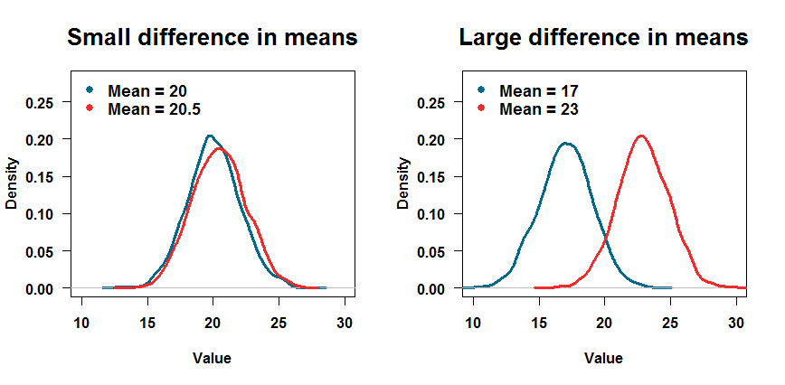
One of the biggest benefits, though, is how easy it is to test ideas. Let’s say, for example, that you learned about t-tests in a stats class. The test theoretically makes sense, but you want a way to visualize what it really means when you compare two samples. In R, you can easily create random data, so you can create the conditions under which two samples should be significantly versus non-significantly different. You know what you’re putting in, so you can see what comes out. This will prepare you for how to look at real data later. It’s easy to visualize data in R, so you can look at what you’re trying to do.
| R |
1
2
3
4
5
6
7
8
9
10
# Create samples by drawing from two normal distributions
sample1 <- rnorm(15, 20, 2)   # N = 15, mean = 20, sd = 2
sample2 <- rnorm(15, 20.5, 2) # N = 15, mean = 20.5, sd = 2

# Plot the two distributions
plot(density(sample1), lwd = 2, col = "deepskyblue4")
lines(density(sample2), lwd = 2, col = "firebrick2")

# Are the means significantly different?
t.test(sample1, sample2)
How does the p-value change if you have more data in each sample? Change the 15s to 100s in lines 2-3 above, rerun the code, and you’re done. What if the two distributions are further apart from each other? Change the means in lines 2-3 above, rerun the code, and you’re done. You don’t have to trust some guy on the internet telling you what to believe; R lets you test things yourself.
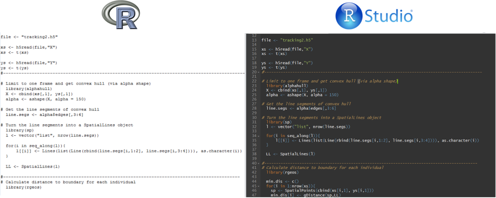
When you program, you leave behind a trail of code that leads to the result or visualization you produced. With a bit of practice, it’s easy to share code, meaning others can replicate your analysis. The code for the above plots, for example, is at the end of this blog post.
Do I have to pay for R? How do I get it?
R is free. You can download it from the R website. I infinitely recommend also downloading R Studio, an interface that makes R easier to use. It organizes your windows (so plots are always in the same place, for example) and highlights the syntax so it’s easier to read.
Why is R free?
According to this Quora thread, there are a few major reasons some programming languages are free. For R (and Python), being free and open-source is a big welcome mat for others to trust the software and start using it. (Open-source means the code is visible and anyone can submit changes to improve it. Here is the source code for R.) R was created by two statisticians at the University of Auckland, New Zealand, so it’s likely to be open-source so it’s easier for other academics to collaborate and exchange analyses. It’s no use having some great statistical software that no one else trusts or can use!
I took a class in college that used MATLAB, so I’ll just keep using that.
Sure, go ahead. However, note that coding languages like MATLAB, Mathematica, SPSS, SAS, and Stata all require paid licenses. It’s unlikely to be a problem if you’re a grad student at a well-funded university, but don’t code yourself into a corner: many industry jobs don’t want to pay the tens of thousands of dollars for a license, so it might be a safer bet to learn a free software like R or Python. [I actually know someone who interviewed at Facebook for a data scientist position, and they wouldn’t accept MATLAB as a coding language – only R or Python.]
This sounds like an advertisement for R.
I believe R made me into a much better scientist, and I’m a big fan!
So why do you use R?
R is (currently) unparalleled in its ability to easily run complicated statistical tests and to produce beautiful data visualization. Instead of coding a non-linear least squares regression from scratch, you can download R code that’ll do it for you. Similarly, investing a little time into learning how R plots data can let you produce almost any visualization you can imagine. And as I mentioned before, R’s community is sufficiently large that websites like Stack Overflow constantly have people asking and answering questions about how to code something in R. 99% of my solutions to R questions come from searching through this community.
However, note that R shines most strongly for statistics and data visualization. With simplicity and ease of use comes some computational inefficiency. If you really want to get into computation-heavy fields like video game development, autonomous cars, or large-scale immunology simulations, check out C instead. As for how R compares to Python for data science and data analytics, DataCamp posted a useful comparison for R and Python’s strengths and weaknesses.
[Side note: I coded exclusively in R when I wrote this post in 2015. Since finishing my Ph.D., I’ve migrated over to Python, but I still love R for its simplicity for analyses. Check out the “Perspectives on Python after R” post for a deep dive on the languages’ differences.]
So I downloaded R. How do I do anything?
If you’re coming from click-based programs like Excel or SPSS, seeing a program that’s just a command line can be a bit of a shock. Think of R as a language and less as a program. Of course you can’t say anything in German when you start learning, or mastering all the tones in Mandarin can be frustrating (or hilarious).
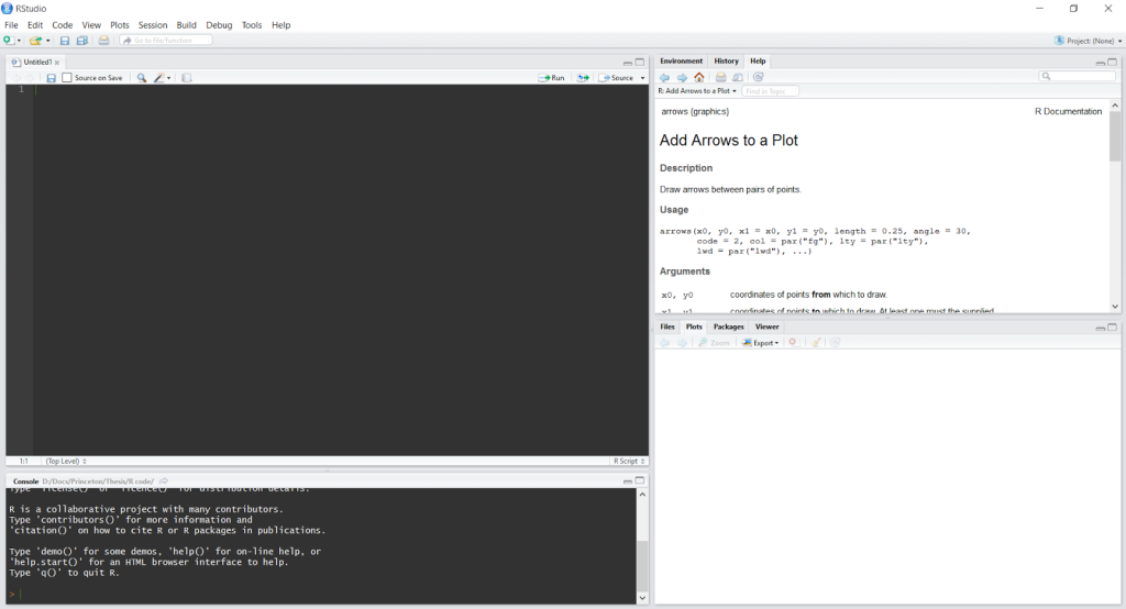
Hopefully you’re in RStudio right now. In the TOP LEFT window, you can type whatever you want, and hitting enter doesn’t make R run the code. This allows you to write several lines of code before you run anything, which is essential for more elaborate programming. To run a line of code in this window, press ctrl + r on Windows or ctrl + ENTER on Mac.
The BOTTOM LEFT window is the terminal, where you can talk directly to R. When you open RStudio, there’s some text here about R and what version you have. Typing here and then pressing ENTER makes R run what you wrote. This is nice if you just want to type a quick command to check something, e.g. what x is equal to. For now, let’s focus on this window.
(The TOP RIGHT window is useful for having extra information about commands, like what arguments they take. For me, the BOTTOM RIGHT window displays plots.)
Below are the very first things you should do in R before you try any data analysis. This code can be copied directly into R and run.
| R |
1
2
5
5 + 5
Yes, literally just type the number 5 into that box in the bottom of the screen and hit enter. Unsurprisingly, R says 5 back to you, confirming that 5 = 5 after all. Now try 5 + 5. Great work.
| R |
1
2
x <- 5
x
The arrow <- is the equals sign in R. (You can use an actual equals sign if you want, but essentially everyone uses the arrow.) By typing x and hitting ENTER, you’ve made a variable x that has the value 5. R will remember this until you tell it to forget, or you close R. Now if you ask R to tell you what x is, it will say 5.
Commands in R
Congratulations; you’ve just coded! If you want the formal introduction to coding, though, you’re supposed to type this:
| R |
1
print("Hello, world!")
print is a command that, well, prints whatever is inside the parentheses. It’s straightforward when you’re printing literally what’s inside of the command, but we can make it more interesting like this:
| R |
1
2
y <- 5
print(y)
Another critically important function to know is the concatenate function, or c. When you use c, you can save multiple elements to a variable, for example creating a vector of numbers instead of just one number.
| R |
1
2
z <- c(1, 2, 4, 8)
z
We can now run some standard analyses on that vector.
| R |
1
2
3
4
5
mean(z)
median(z)
sd(z)
min(z)
max(z)
We could also just run it directly on the numbers if you’d prefer.
| R |
1
mean(c(1, 2, 4, 8))
Loading data into R
This one caused me so much confusion when I was first learning R. It involves thinking a bit like a computer.
Step 1: Save the data in a format R will understand
This post from R Bloggers goes into intricate detail on all the file formats R will accept and how to load them. If your data is in Excel, one of the simplest ways to load it into R is to use the .CSV format, which stands for “comma-separated values.”
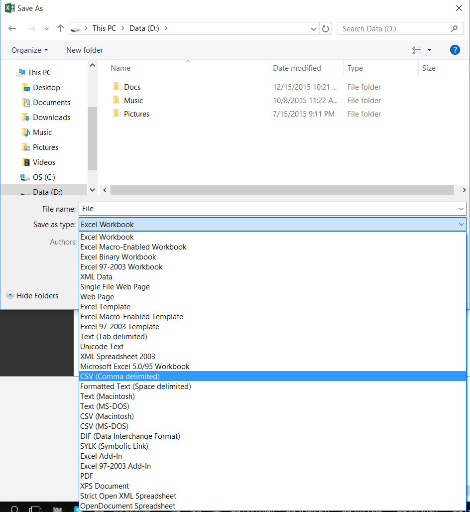
Say you have an Excel spreadsheet that you want to open in R. In Excel:
- Make sure there are no spaces in the column names. Changes the names from e.g.
Time (seconds)toTime_sec. File->Save As->Save as Type->CSV (Comma delimited)- Excel will say some features of the workbook may be lost. Say that Yes, you do want to keep using the CSV format.
- When you exit, it will ask if you want to save your changes. Go ahead and save, even if you didn’t make any changes.
Step 2: Specify the working directory in R
Now you will need to tell R where to find the data. When you use a programming language, it focuses on one particular folder in your computer at a time, and you have to tell it which folder to look at. This folder is called the working directory. You can find out where you currently are by typing getwd(). You can change the working directory with the setwd command. If you’re on a Windows computer, your data file is in the Desktop, and your username is Matt, you can type this to get to the Desktop:
| R |
1
setwd("C:/Users/matt/Desktop")
Step 3: Load the data
This step will involve creating a variable called data and assigning to it the output of the read.csv function.
| R |
1
data <- read.csv("Data.csv", header=T)
If there’s a file called Data.csv on the Desktop, R will load it using the read.csv command and assign the data to the variable data. The header=T argument tells R that the top row of the data is column names. (If you just imported a table of numbers with no header, for example, you could say header=F instead.)
Step 4: Look at the data
Now you can look at the data. You could just type data and hit enter, but then R will display everything, so if you have more than a little data, your screen will become overwhelmed by numbers. A better option is to display only part of the data.
| R |
1
2
3
head(data)
tail(data)
data[1:5, c(2,4)]
The head and tail commands tell R to only look at the first or last 6 rows of the data.
The last command, data[1:5, c(2,4)], offers you more fine-tuned control. The brackets [] let you subset the data, which means selecting only part of it. The first argument, 1:5, means “rows 1 through 5.” The second argument, c(2,4), means “columns 2 and 4.” You always list rows first, then columns.
If you wanted to create a new variable for all rows but only columns 1, 3 to 5, and 7 of the data, you could write something like this:
| R |
1
new_data <- data[, c(1, 3:5, 7)]
The first empty argument means “all rows.”
Finally, here are three commands to get a feel of the data.
| R |
1
2
3
dim(data)
summary(data)
str(data)
dim will tell you the dimensions of the data, i.e. how many rows and columns there are. summary will summarize each column in the data, giving you values like the first quartile, median, etc. str gives you the structure of the data, telling you what type of data each column has (e.g. integers, factors, characters).
I still don’t know how to do anything in R.
That’s ok. Again, think of R as a language instead of a program. It takes a while to gain fluency, but the more you invest in learning, the easier it’ll be to say what you’re thinking.
One of the most important things for me when I first started learning R was to learn where to find answers to my questions. Let’s say you found a function but don’t know how to use it.
| R |
1
?mean
This will bring up R’s Help file for the mean function. There you can find what the function does, as well as what arguments R is looking for.
Say you don’t know what the function is called in R. Let’s say you’re trying to find the command for standard deviation:
| R |
1
??"standard deviation"
This will search R’s Help files and return functions whose help files contain the words “standard deviation.” The stats::sd option is what you’re looking for. stats refers to the package in R, and sd is the command. (A package is a collection of functions and variables that you can optionally load for specific analyses. stats is actually one of the defaults loaded by default any time you start R.)
Finally, say you’re looking for a function for standard error and ??"standard error" only gives you complicated-sounding options that don’t seem right. Now it’s time to type the following into Google: standard error in R.
The first link, unsurprisingly, takes you to Stack Overflow, where someone asked this exact question in 2011. The answer is that R doesn’t have a function for standard error, but it’s really easy to write one. I’ll cover writing your own functions in a future post. When in doubt, Google what you’re trying to do, followed by “in R”. Honestly, this is usually the easiest way to find what you’re looking for.
What are other resources for learning R? No offense.
None taken. Here are some invaluable resources that have helped me learn.
This book was exactly what I needed when I was first learning R. I needed something for an absolute beginner, and this book helped me overcome that initial learning curve.

Quick-R provides an incredibly useful overview of basic functions in R. I visit their page on graphical parameters all the time.

The posts at R-bloggers are incredibly helpful. While they won’t necessarily provide the well-rounded introduction to R you might need, they’re very useful for coding a random, specific analysis that might be hard to find elsewhere. A 2005 post on shading a polygon was exactly what I needed for the analysis in this blog post. I follow them on Twitter and will read the occasional article that pops up and is relevant to me.

I’ve never gone to their website directly, but I always end up there from Googling questions about R. It’s such an easy way to learn how to run a particular analysis in R. Google your question and then see if it’s already been answered on Stack Overflow.
Thanks for reading! This is the first post in a series on R. The next post will be on plotting and simple statistical tests.
Best,
Matt
Code for the figures in this post
| R |
1
2
3
4
5
6
7
8
9
10
11
12
13
14
15
16
17
18
19
20
21
22
23
24
25
26
27
28
29
30
31
32
33
34
35
36
37
38
39
40
41
42
43
44
45
46
47
48
49
50
51
52
53
54
55
56
57
# Create the distributions. Start by listing the parameters up top. All
# groups will be drawn from a normal distribution with standard
# deviation = 2. We'll sample 2000 values to make the distributions
# nice and smooth.
N <- 2000
sd <- 2

# The means, however, will differ between groups
mean1 <- 20
mean2 <- 20.5
mean3 <- 17
mean4 <- 23

# Now we actually create the distributions
sample1 <- rnorm(N, mean1, sd)
sample2 <- rnorm(N, mean2, sd)
sample3 <- rnorm(N, mean3, sd)
sample4 <- rnorm(N, mean4, sd)

# Plot the figures
# First, divide the graphics window into 1 row, 2 columns
par(mfrow = c(1,2))

# Figure 1: small difference in means
plot(density(sample1), lwd = 3, las = 1,
    col = "deepskyblue4",
    xlim = c(10, 30), ylim = c(0, 0.28),
    main = "Small difference in means",
    cex.main = 1.6, xlab = "Value",
    font.axis = 2, font.lab = 2)
lines(density(sample2), lwd = 3, col = "firebrick2")

# Add a legend with bolded text
par(font = 2)
legend("topleft", bty = 'n', pch = 19,
    col = c("deepskyblue4", "firebrick2"),
    legend = c(paste0("Mean = ", mean1),
               paste0("Mean = ", mean2)),
    cex = 1.1)

# Figure 2: a large different in means
plot(density(sample3), lwd = 3,
    col = "deepskyblue4",
    xlim = c(10, 30), ylim = c(0, 0.28),
    main = "Large difference in means",
    las = 1, cex.main = 1.6, xlab = "Value",
    font.axis = 2, font.lab = 2)
lines(density(sample4), lwd = 3,
    col = "firebrick2")

# Add a legend with bolded text
par(font = 2)
    legend("topleft", bty = 'n', pch = 19,
    col = c("deepskyblue4", "firebrick2"),
    legend = c(paste0("Mean = ", mean3),
               paste0("Mean = ", mean4)),
    cex = 1.1)