
Learning R 4. Functions and if statements
#r
Written by Matt Sosna on May 15, 2016
Learning R series
- Introduction
- Random data and plotting
forloops and random walks- Functions and
ifstatements - The
applyfunctions
If you’ve been following this series from the first post, you might recall this soapbox speech I gave:
With programming, you get rid of the comfortable structure of a friendly interface with buttons in favor of freedom. Your analyses are now limited by your imagination and knowledge of the R language, not what someone else thought was relevant for you.
I immediately contradicted that quote with three posts full of using R’s built-in functions, which some developer at R “thought was relevant for you”… but it was all part of the grand plan! Now that we’re comfortable with some R fundamentals, let’s start really carrying out the meaning behind that quote above. In this post, we’ll “customize” our code by taking hold of the tools to write our own functions. We’ll also get started with control flow (if and else statements) and logical operators (&, |, etc.).
This is the fourth in a series of posts on R. This post covers:
- Creating your own functions
ifstatements- Logical operators
- Integrating functions and
ifstatements intoforloops
The most important code from previous posts is shown below.
| R |
1
2
3
4
5
6
7
8
9
10
11
12
13
14
15
16
17
18
19
20
21
22
c()            # Concatenate
x <- c(5, 10)  # Assign the vector (5, 10) to the variable "x"
x[x > 7]       # Subset the values of x that are greater than 7

# Assign 100 randomly-drawn values from a normal distribution with
# mean=0 and sd=1 to the object "data"
data <- rnorm(100)

# Plot a histogram of the data
hist(data)

# Assign 100 randomly-drawn values from a uniform distribution with
# minimum=0 and maximum=1 to the object "y"
y <- runif(100)

# Plot a scatterplot of the variable "y" as a function of "data"
plot(y ~ data)

# For "i" in the sequence "1 to the length of x", print "i"
for(i in 1:length(x)){
  print(i)
}
Creating functions
A function is basically a box with some machinery inside. You give a function an input, the box rumbles around for a bit, and then it returns an output. Here’s an example of a simple mathematical function:
\[f(x) = x + 1\]Here, \(f(x)\) is the output and \(x\) is the input. If your input is 5, the function looks like this:
\[f(x) = x + 1\] \[f(5) = 5 + 1\] \[f(5) = 6\]In R, we can give this function a name and then call it later.
| R |
1
add_one <- function(x){x + 1}
add_one is the name of our function. Above, function is the command in R that says “Assign the instructions inside the curly brackets to the variable add_one.” Similarly to how for loops find wherever you wrote an i and replace it with a number, add_one will replace x with whatever you feed into it. (You also don’t have to use x. The alternate function(N){N + 1} is identical to our add_one.)
What’s nice about writing a function is that now you can just say add_one(5) or add_one(1:1000) and R will run your inputs (here: 5 and 1:1000 (1, 2, 3, … , 1000) through that equation for you. And if you ever forget the code that went into creating this function, just type add_one and R will print out the code inside the function.
[I find this ability to print out the contents of a custom function to be a nice contrast to Python, which only returns the address in memory (or some user-defined strings if you tinker with magic methods).]
Our own mean function
Here’s something slightly more complicated. R has a built-in function for finding the mean of a vector or matrix, but we can easily write our own version.
| R |
1
our_mean <- function(x){sum(x) / length(x)}
We can check it by creating a vector with some values and comparing the outputs from R’s mean and our own.
| R |
1
2
3
values <- seq(from = 4, to = 6, by = 0.5)
our_mean(values)   # 5
mean(values)       # 5
More advanced mechanics
You are essentially unhindered in what you make into a function. You can have multiple inputs that interact with each other, you can specify default values, you can nest functions within each other… let your imagination go wild.
| R |
1
2
3
4
5
6
7
multiply <- function(x, y){x * y}
multiply(5, 1:5)  # 5 10 15 20 25

mega_multiply <- function(x, y){multiply(x, y) * x * y}
mega_multiply(1e5, 1e-5)  # 1

super_duper <- function(x, y, z = 1){ (x + y) / z }
In super_duper, the x and y inputs are required, but z is optional. If you don’t include z, R will automatically set z = 1. Conversely, if you write function(x, y, z) and then don’t specify z when you call the function (e.g. super_duper(1, 1)), R will raise an error.
if statements
Let’s say you want R to run a command only if a certain condition is met. You’re curious if 1 + 1 is less than 5, for example, because you skipped that day of kindergarten and you’re finally ready to address this gap in your knowledge… using R.
| R |
1
if(1 + 1 < 5){print("Yup, less than 5")}
R will print the statement only if 1+1 is less than 5. To avoid spoilers, I won’t post the output from R; it’s on you to figure this one out! ;-)
We can easily turn this if statement into a function that checks whether any input is less than 5:
| R |
1
2
3
less.than.five <- function(x){if(x < 5){return("Yup, less than 5")}}
less.than.five(3)  # Yup, less than 5
less.than.five(10) # NULL
Note that we include return in our function now. For functions with only one calculation, we can get away without explicitly telling R to return the output. But especially as we start creating functions with multiple commands, we’ll want to make sure we’re including return - it’ll help anyone reading your function to better understand what’s going on.
Also note that nothing happens when the input to less.than.five is greater or equal to five. That’s because we didn’t tell R what to do if this situation occurs, so it does nothing. (This sort of logic flow - not doing something if a condition isn’t met - is useful in a script, but we don’t want our functions to sometimes return strings and sometimes return NULL. Here, a little extra code that handles cases where \(x == 5\) or \(x > 5\):
| R |
1
2
3
4
5
less.than.five <- function(x){
  if(x < 5){
    return("Yup, less than 5")} else if (x == 5) {
    return("No, it's 5")} else {
    return("No, greater than 5")}}
In English, this reads as:
- If
x< 5, return “Yup, less than 5.” - If
xis not less than 5, check ifxis 5. If it is, return “No, it’s 5.” - If neither of the previous conditions were met, return “No, greater than 5.”
The else if statement is another if statement that only executes if the previous if statement evaluated to False.
- First
if: True or False?- True -> skip the
else if - False -> execute the
else if
- True -> skip the
This is in contrast to having two if statements in a row, whose logic would flow like this:
- First
if: True or False?- Doesn’t matter, second
ifexecutes either way
- Doesn’t matter, second
Finally, the else statement tells R that if neither of the previous if statements were met, execute the code inside its curly brackets.
A brief tour of logical operators
In line 4 above, we use x == 5 because that notation asks R if the statement is true or false. If we wrote x = 5, we’d be assigning the value 5 to x, which causes an error within the if statement. You can use the logical operators <, >, <=, >=, ==, |, &, and ! to ask R if a statement is true.
| R | English |
|---|---|
x == 4 |
x equals 4, true or false? |
x != 4 |
x does not equal 4, true or false? |
x > mean(c(10, 4)) |
x is greater than the mean of 10 and 4, true or false? |
x < 4 | x > 2 |
x is less than 4 OR x is greater than 2, true or false? |
x < 4 & x > 2 |
x is less than 4 AND x is greater than 2, true or false? |
Integrating function, if, and for loops
In the previous R post, we talked about for loops and random walks. Much like a frustrating cumulative exam in school, let’s incorporate everything we’ve learned to answer a tougher question: how do we write a function that finds the median?
 No, using R’s built-in
 median function won’t cut it in this tutorial. Let’s write our own. (median does, however, serve as a nice check to see whether our function is doing what we think it is.)
As a brief review of summary statistics, when we have a set of numbers, we often want a description of the “average” value of the set, or what we would expect if we drew a random value. Common descriptors are the mean, median, and mode. The median is the value that divides the set such that half of the values are below the median, and half are above. The median doesn’t care about the actual values in the set; it will just find the middle-ranked one. It’s therefore insensitive to outliers that would otherwise wreck the output from the mean. (If Bill Gates visited a high school classroom, the mean income of the people in the classroom would skyrocket to millions of dollars, while the median - the income of one of the students - would be a better representation of the average income in the room.)
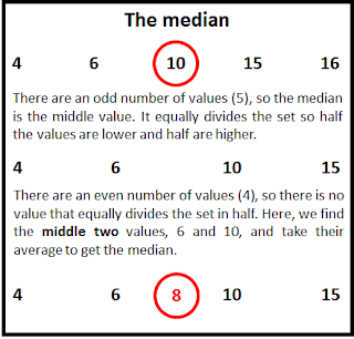
There are a few steps to finding the median. Let’s write them here to clarify the plan of attack. We start with a set of values. Then:
- Sort the values from lowest to highest
- If there are an odd number of values, the middle value (where an equal number of values lie above and below this point) is the median
- If there are an even number of values, find the middle two values. The mean of these values is the median.
This is how the above would look like in R:
| R |
1
2
3
4
5
6
med <- function(x){
    if(length(x) %% 2 == 1){
        return(sort(x)[length(x) / 2 + 1/2])
    }
    return(mean(sort(x)[c(length(x) / 2, length(x) / 2 + 1)]))
}
A more detailed explanation:
| R |
1
2
3
4
5
6
7
8
9
10
11
12
13
14
15
16
17
18
19
20
21
22
23
24
25
26
27
28
29
30
31
32
33
34
# Define a function called med that takes one input
med <- function(x){

    # If the number of values divided by 2 has a remainder of 1
    # (i.e. there is an ODD number of values)...
    if(length(x) %% 2 == 1){

        return(
            # ...sort the values from lowest to highest and find
            # the value that...
            sort(x)[

            # ...is 1/2 + the length of the input divided by 2
            # (i.e. the middle)
            length(x)/2 + 1/2

            ])}  # close the subset, return, and if statements

    # No second if statement needed because you can only reach this
    # code if length(x) %% 2 == 0 (i.e. there is an EVEN number of
    # values)

    return(
        # Get the mean...
        mean(
            #... of the sorted values subsetted on...
            sort(x)[

            #... the middle value and the next value
            c(length(x)/2, length(x)/2 + 1)

            ]))          # Close the subset, mean, return

} # Close the entire function
Combining all that with a for loop
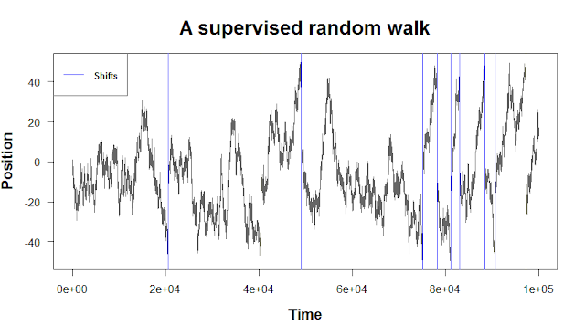
Nice work! Finally, let’s create a one-dimensional random walk that uses if statements and our median function. Let’s say we want to impose boundaries on our random walk such that if it wanders too far from the origin, we restart it at the median of the walk so far.
| R |
1
2
3
4
5
6
7
8
9
10
11
12
13
14
15
16
17
18
19
20
21
22
23
24
25
26
27
28
29
30
31
32
33
34
35
36
37
38
39
40
# Set the parameters
n.steps <- 1e5    # 100,000 steps (1.0 x 10^5)
mean.step <- 0    # Walk is unbiased (no preference up or down)
sd.step <- 0.5    # Standard deviation of step sizes (steps drawn
                  # from a normal distribution)
up.boundary <- 50     # The upper boundary of our walk
down.boundary <- -50  # The lower boundary

# Initialize variables
walk <- 0         # Start the walk at zero
shifts <- c()     # Create an empty variable to store time points
                  # when the walk hits a boundary

# The random walk
for(i in 2:n.steps){

    # First, take a step
    walk[i] <- walk[i-1] + rnorm(1, mean.step, sd.step)

    # If the walk stepped out of bounds...
     if(walk[i] > up.boundary | walk[i] < down.boundary){

        # ...reset the walk at the median value of the walk so far
        walk[i] <- med(walk)

        # Record when the walk stepped out of bounds
        shifts[i] <- i
    }

    # Display the iteration
    print(i)
}

# Plot it
plot(walk, type = 'l', main = "A supervised random walk", las = 1,
     xlab = "Time", ylab = "Position", cex.main = 1.8, cex.lab = 1.4,
     font.lab = 2, col = "gray40")
abline(v = shifts, col = "blue")
par(font = 2)
legend("topleft", lty = 1, col = "blue", legend = "Shifts", cex = 0.8)
Thanks for reading. In the next post, we’ll cover the apply functions, which are convenient methods for performing many calculations at once.
Cheers,
Matt