
How to enter data science 3. The analytics
#careers
#data-science
#machine-learning
#python
Written by Matt Sosna on December 15, 2020
Welcome to the third post in our series on how to enter data science! The first post covered how to navigate the broad diversity of data science roles in the industry, and the second was a deep dive on (some!) statistics essential to being an effective data scientist. In this post, we’ll cover skills you’ll need when manipulating and analyzing data. Get ready for lots of syntax highlighting!
How to enter data science:
- The target
- The statistics
- The analytics
- The engineering
- The people
Code for days
While Excel wizardry might cut it for many analytics tasks, data science work relies heavily on the nuance, reproducibility, and scalability of programming. From statistical tests only available in specialized R and Python libraries, to being able to show step-by-step how a model is formulated and generates predictions, to being able to go from processing one dataset to 1,000 with a few keystrokes, fluency in programming is essential for being an effective data scientist. We’ll therefore focus on programming skills that are key to effectively manipulating and analyzing data. These skills should prove useful no matter where your role is on the analytics-engineering spectrum.
While plenty of data science roles rely solely on R, this post will demonstrate coding concepts with Python. Python’s versatility makes it an “all-in-one” language for a huge range of data science applications, from dataframe manipulations to speech recognition and computer vision. Even if your role involves crunching numbers all day in R, consider learning a little Python for automating steps like saving results to your company’s Dropbox.
This post assumes you’re familiar with Python basics. If not, check out the great material at Real Python and Codecademy.
Here are the technical skills we’re covering in this series. Inferential statistics is covered in the last post, analytics in this post, and software engineering in the next post.
- Inferential Statistics
- Experimental design
- Comparisons between groups
- Predictive modeling
- Model internals
- Analytics
- Dataframes
- Arrays
- Visualizations
- Descriptive statistics
- Working with dates and time
- Machine learning
- Software engineering
- Accessing data
- Version control
- Object-oriented programming
- Virtual environments
- Writing tests
Dataframes
Dataframes are at the core of data science and analytics. They’re essentially just a table of rows and columns, typically where each row is a record and each column is an attribute of that record. You can have a table of employees, for example, where each row is a person and the columns are their name, home address, and job title. Because dataframes play a central role in data science, you’ll need to master visualizing and manipulating the data within them. pandas is the key library here.
The basics include being able to load, clean, and write out CSV files. Cleaning data can involve removing rows with missing values or duplicated information, correcting erroneous values, and reformatting columns into different data types.
| Python |
1
2
3
4
5
6
7
8
9
10
11
12
13
14
15
16
17
import os
import pandas as pd

# Load the data
os.chdir("~/client/")
df = pd.read_csv("data.csv")

# Fix issues with 'state' column
df['state'].replace({'ill': 'IL', 'nan': None}, inplace=True)
df_filt = df[df['state'].notna()]

# Remove duplicates and reformat columns
df_filt = df_filt.drop_duplicates(['customer_id', 'store_id'])
df_filt = df_filt.astype({'price': float, 'age': int})

# Save data
df_filt.to_csv("cleaned.csv", index=False)
Other important data manipulations include vectorized and iterative data transformations. For simple elementwise math on columns in our dataframe, pandas lets us treat the columns as if they were singular values.
| Python |
1
2
3
# Simple vectorized transformations
df['added'] = df['col1'] + df['col2']
df['multiplied'] = df['col1'] * df['col2']
For more nuanced operations, such as handling missing values that would otherwise cause columnwise operations to fail, you can use .apply. Below, we use a lambda to apply a custom function, safe_divide, to the col1 and col2 fields of each row.[1]
| Python |
1
2
3
4
5
6
7
8
9
10
11
12
13
# Define a custom function
def safe_divide(x, y):
    """
    | Divide x by y. Returns np.nan if x or y are null
    | or y is zero.
    """
    if pd.isna([x, y]).any() or y == 0:
        return np.nan
    return x / y

# Apply it to our df
df['divided'] = df.apply(lambda x: safe_divide(x['col1'], x['col2']),
                         axis=1)
For logic that can’t be easily passed into a lambda, we can iterate through the dataframe rows using .itertuples. (Don’t use .iterrows if you can avoid it!)
| Python |
1
2
3
4
5
6
7
8
9
10
11
12
13
# Instantiate a df to append data to
df_final = pd.DataFrame()

# Iterate through the rows of our df
for tup in df.itertuples():

    # Logic that can't easily be passed into a lambda
    if tup.Index % 2 == 0 and tup.is_outdated:
        df_iter = some_function(tup.age, tup.start_date)
    else:
        df_iter = some_other_fuction(tup.age, tup.pet_name)

    df_final = df_final.append(df_iter, ignore_index=True)
Finally, we need the ability to combine data from multiple dataframes, as well as run aggregate commands on the data. In the code below we merge two dataframes, making sure not to drop any rows in df1 by specifying that it’s a left merge. Then we create a new dataframe, df_agg, that sums each column for each user. Since user_id is now our index, we can easily display a specific user’s spending in a given category with .loc.
| Python |
1
2
3
4
5
6
7
8
9
10
11
12
13
14
15
16
# Merge data, avoiding dropping rows in df1
df_merged = pd.merge(df1, df2, on='user_id', how='left')

# Preview the data
df_merged.head()
# user_id   groceries   utilities   video_games
#  123      100         100         5000
#  123      200         0           9999
#  456      0           1e6         0
#  ...      ...          ...        ...

# Sum all numerical columns by user
df_agg = df_merged.groupby('user_id').sum()

# Display user 123's grocery spending
print(df_agg.loc[123, 'groceries'])  # 300
Arrays
pandas dataframes are actually built on top of numpy arrays, so it’s helpful to have some knowledge on how to efficiently use numpy. Many operations on pandas.Series (the array-like datatype for rows and columns) are identical to numpy.array operations, for example.
numpy, or Numerical Python, is a library with classes built specifically for efficient mathematical operations. R users will find numpy arrays familiar, as they share a lot of coding logic with R’s vectors. Below, I’ll highlight some distinctions from Python’s built-in list class. A typical rule of thumb I follow is that it’s better to use Python’s built-in classes whenever possible, given that they’ve been highly optimized for the language. In data science, though, numpy arrays are generally a better choice.[2]
First, we have simple filtering of a vector. Python’s built-in list requires either a list comprehension, or the filter function plus a lambda and unpacking ([*...]). numpy, meanwhile, just requires the array itself.
| Python |
1
2
3
4
5
6
7
8
9
10
11
12
13
import numpy as np

# Create the data
list1 = [1, 2, 3, 4, 5]
array1 = np.array([1, 2, 3, 4, 5])

# Filter for elements > 3
## The list way
[val for val in list1 if val > 3]  # [4, 5]
[*filter(lambda x: x > 3, list1)]  # [4, 5]

## The numpy way
array1[array1 > 3]   # array([4, 5])
A second major distinction is mathematical operations. The + operator causes lists to concatenate. numpy arrays, meanwhile, interpret + as elementwise addition.
| Python |
1
2
3
4
5
6
7
8
9
10
11
12
# Create the data
list1 = [1, 2, 3]
list2 = [4, 5, 6]
array1 = np.array([1, 2, 3])
array2 = np.array([4, 5, 6])

# Addition
## Lists: concatenation
list1 + list2   # [1, 2, 3, 4, 5, 6]

## Arrays: elementwise addition
array1 + array2 # array([5, 7, 9])
To do elementwise math on Python lists, you need to use something like a list comprehension with zip on the two lists. For numpy, it’s just the normal math operators. You can still get away with manually calculating simple aggregations like the mean on lists, but we’re nearly at the point where it doesn’t make sense to use lists.
| Python |
1
2
3
4
5
6
7
8
9
10
# Elementwise multiplication
## Lists: list comprehension
[x * y for x, y in zip(list1, list2)]  # [4, 10, 18]

## Arrays: just the * operator
array1 * array2  # array([4, 10, 18])

# Get the mean of an array
sum(list1)/len(list1)  # 2.0
array1.mean()          # 2.0
Finally, if you’re dealing with data in higher dimensions, don’t bother with lists of lists - just use numpy. I’m still scratching my head trying to figure out how exactly [*map(np.mean, zip(*l_2d))] works, whereas arr_2d.mean(axis=1) clearly indicates we’re taking the mean of each column (axis 1).
| Python |
1
2
3
4
5
6
7
8
9
10
11
12
# List of lists vs. matrix
list_2d = [[1, 2, 3],
           [4, 5, 6]]
arr_2d = np.array(list_2d)

# Get mean of each row
[np.mean(row) for row in list_2d]  # [2.0, 5.0]
arr_2d.mean(axis=1)                # array([2.0, 5.0])

# Get mean of each column
[*map(np.mean, zip(*l_2d))]   # [2.5, 3.5, 4.5]
arr_2d.mean(axis=0)           # array([2.5, 3.5, 4.5])
If you end up working in computer vision, numpy multidimensional arrays will be essential, as they’re the default for storing pixel intensities in images. You might come across a two-dimensional array with tuples for each pixel’s RGB values, for example, or a five-dimensional array where dimensions 3, 4, and 5 are red, green, and blue, respectively.
Visualizations
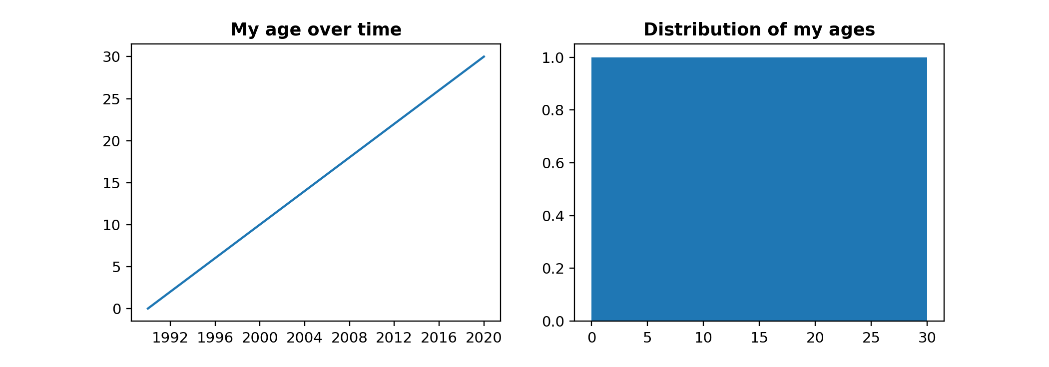
After dataframes and arrays, the next most crucial analytics skill is data visualization. Visualizing the data is one of the first and last steps of an analysis: when Python is communicating the data to you, and when you’re communicating the data to stakeholders. The main Python data visualization libraries are matplotlib and seaborn. Here’s how to create a simple two-panel plot in matplotlib.
| Python |
1
2
3
4
5
6
7
8
9
10
11
12
13
14
15
16
import matplotlib.pyplot as plt

# Set figure size
plt.figure(figsize=(10, 4))

# Subplot 1
plt.subplot(1,2,1)
plt.plot(df['date'], df['age'])
plt.title('My age over time', fontweight='bold')

# Subplot 2
plt.subplot(1,2,2)
plt.hist(df['age'], bins=31)
plt.title('Distribution of my ages', fontweight='bold')

plt.show()
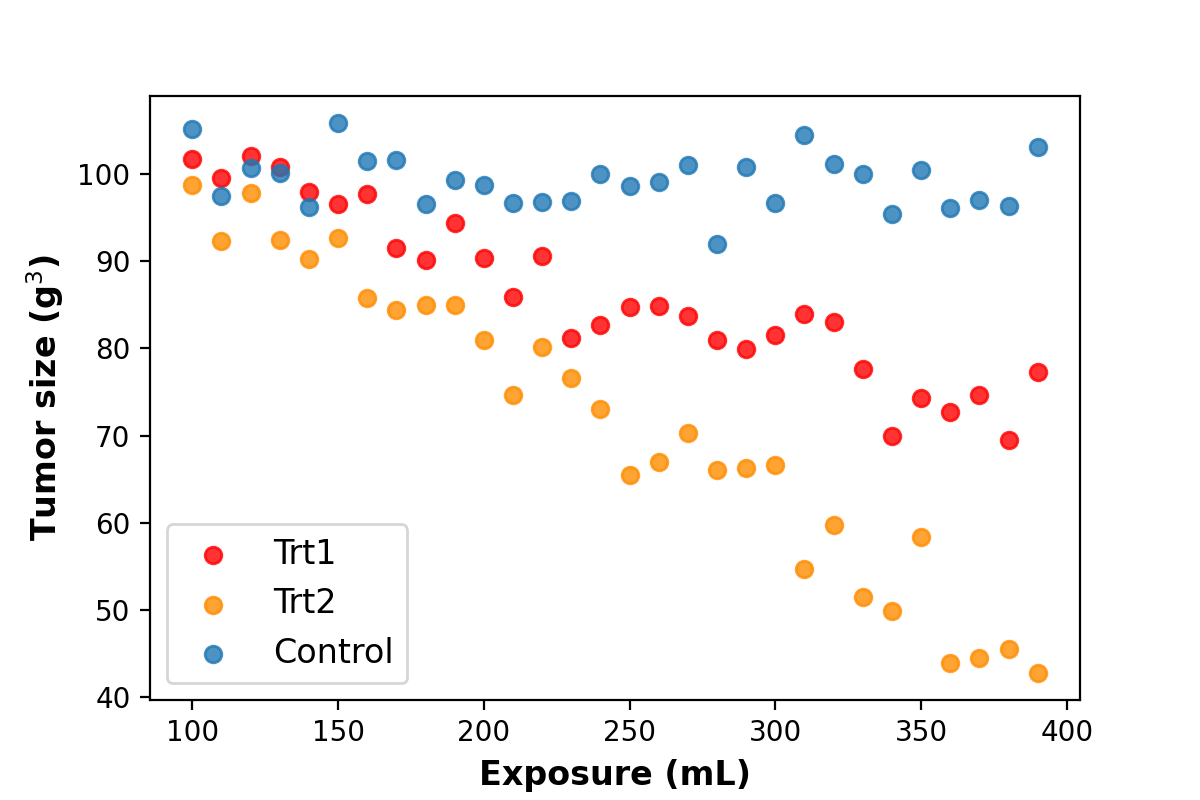
And below is a simple way to plot data with multiple groups. The label keyword is incredibly handy, as you can then simply call plt.legend and auto-populate the legend with info on each group.
| Python |
1
2
3
4
5
6
7
8
9
10
11
12
13
14
# Define dict for colors
trt_dict = {'Trt1': 'red', 'Trt2': 'darkorange', 'Control': 'C0'}

# Iteratively add data to a plot
for trt in df['treatment'].unique():
    df_trt = df[df['treatment'] == trt]
    plt.scatter(df_trt['exposure'], df_trt['tumor_size'], label=trt,
                color=trt_dict[trt], alpha=0.8)

plt.xlabel('Exposure (mL)', fontweight='bold', fontsize=12)
plt.ylabel('Tumor size (g$^3$)', fontweight='bold', fontsize=12)
plt.legend(fontsize=12)

plt.show()
If you want to get fancy, look into interactive dashboarding tools like Bokeh or Plotly. These tools let the user interact with the plot, such as getting more information about a point by hovering over it, or regenerating data in the plot by clicking on drop-down menus or dragging sliders. You can even embed simple plots into static HTML, like the Bokeh plot below.[3]
Descriptive statistics
While you may be chomping at the bit to get to machine learning, I think a solid understanding of descriptive statistics should come first. (As well as inferential statistics if you skipped the last post!) The basics should be enough for most data science applications.
In contrast to inferential statistics, which involves translating data on our sample to inferences about a broader population, descriptive statistics involves summarizing the data you have. Is the data normally distributed, unimodal or bimodal, skewed left or right? What’s a typical value, and how much do the data vary from that value? Think of descriptive stats as the “hard numbers” pair to data visualization. Being able to quickly communicate these metrics will provide an intuition for the data that helps identify outliers, such as data quality issues.
Here are the main metrics I think are essential to know:
- Averages: mean, median, mode
- Spread: standard deviation
- Modality: unimodal, bimodal, multimodal distributions
- Skew: left, right
| Python |
1
2
3
4
5
6
7
8
9
10
11
12
13
import numpy as np
from scipy.stats import sem, normaltest

# Generate random data
data = np.random.normal(50, 3, 1000)

# Summarize mean and standard error
print(data.mean())  # 50.053
print(sem(data))    # 0.094

# Is the data normally distributed?
print(normaltest(data))
# NormaltestResult(statistic=3.98, pvalue=0.137) -> Yes
Working with dates and time
At least with data analytics, you most likely won’t escape working with dates. Dates form the backbone of time series analysis, which is ubiquitous in fields with continuous data streams like the Internet of Things.
The built-in datetime library is Python’s standard, with expanded methods in the dateutil library. Thankfully, pandas has excellent functionality for working with dates when the index is set to datetime, meaning you can stay in pandas for analyses both with and without dates. Similarly, matplotlib lets you pass in dt.datetime values as if they were normal numbers.
| Python |
1
2
3
4
5
6
7
8
9
10
11
12
13
14
15
16
import pandas as pd
import datetime as dt
from dateutil.relativedelta import relativedelta

# Play with dates
today = dt.date.today()
yesterday = today - dt.timedelta(days=1)
last_year = today - relativedelta(years=1)

# Generate sample data with datetime index
df = pd.DataFrame({'data': [100]*60},
                  index=pd.date_range('2020-01-01', '2020-02-29'))

# Sum the data for each month
df_new = df.resample('MS').sum()
df_new.plot(kind='bar')  # Call built-in matplotlib from pandas
Converting between dt.datetime and str formats will be important as well. The functions here are:
dt.datetime.strptimeforstr->dt.datetimedt.datetime.strftimefordt.datetime->str.
(Note: I still can never remember whether the string or datetime value goes first! I just try it in a Jupyter notebook cell on the side and see which one works.)
| Python |
1
2
3
4
5
6
7
8
# String to datetime
date_str = "2020-01-01 12:00"
date_dt = dt.datetime.strptime(date_str, "%Y-%m-%d %H:%M")
print(date_dt)  # dt.datetime(2020, 1, 1, 12, 0)

# Datetime to string
date_str_new = dt.datetime.strftime(date_dt, "%Y-%m-%d %H:%M")
print(date_str_new)  # "2020-01-01 12:00"
Finally, Python’s time module is handy for timing how long steps in an analysis take. time.time() will return a float representing the number of seconds since midnight on Jan 1, 1970. (Also known as the Unix Epoch time.) You can save this value before a block of code, then compare it to the Epoch time after the code.
| Python |
1
2
3
4
5
6
7
8
9
10
11
12
import time
import numpy as np

start_time = time.time()

# Generate 1 trillion numbers O_O (don't actually do this)
np.random.normal(0, 1, 1e12)

end_time = time.time()

time_in_years = (end_time - start_time)/60/60/24/365
print(f"Duration: {round(time_in_years, 2)} years")
Machine learning
Finally, we have machine learning. Of all the things a data scientist does, machine learning receives the most hype but is likely the smallest aspect of the job.
 Think of being a data scientist as building a huge drilling machine.[4] The drill itself is the eye-catching bit $-$ the fancy statistics and analytics $-$ and the tip is machine learning. The drill tip gets all the credit for breakthroughs, and there are always new and improved drill tips coming out that can break tougher ground.
But the majority of your time will probably be spent building out the rest of the machinery $-$ the frame, levers, screws, etc. $-$ and identifying where to apply the drill. (If you’re in a particularly engineering-strapped organization, you might also end up building the front end: the seat and controls for the user!)
If you only care about the drill instead of the whole machine, you’ll likely find yourself disillusioned by many data science jobs. But if you find enjoyment in the entire process of building the machine and creating something that truly helps people break that ground, then you’ll love your work.
At any rate, you will need some knowledge of machine learning. While you need to understand what any algorithm you use is doing $-$ and whether it’s the right tool for the question you’re asking $-$ you might be surprised how little business mileage you get from studying how exactly similar algorithms differ (e.g. random forests vs. support vector machines vs. XGBoost) unless your role is in research, education, or machine learning consulting.[5] Rather, you’ll get a lot farther if you have a good understanding of the necessary steps before and after you use a machine learning algorithm.
I’ll therefore spend this section on these “before and after” components to using machine learning effectively. The main concepts to know, I’d argue, are:
Feature engineering
Our raw data alone is often not sufficient to build a strong model. Let’s say, for example, that we’re trying to predict the number of items sold each day in an online store. We already know that sales are higher on weekends than weekdays, so we want our model to incorporate a weekday/weekend distinction to be more accurate. A weekday/weekend distinction isn’t explicitly present in our data, though $-$ we just have the date a sale occurred.
A linear model will certainly have no idea what to do with raw dates. Maybe a complex deep learning model can pick up a cyclic pattern in sales related to dates, but it will likely need a lot of data to figure this out.
A much simpler option is to engineer an is_weekend feature by asking whether each sale occurred on a Saturday or Sunday vs. the rest of the week. The is_weekend feature now serves as an unambiguous flag giving our model a heads up that something may be different between weekdays and weekends. Similarly, maybe the raw number of items in users’ shopping carts isn’t an informative predictor, but the square root or logarithm of those items actually is. (I actually have no idea. Send me a message if there’s some transformation all the data scientists in e-commerce use!)
| Python |
1
2
3
4
5
# Create a column for whether the date is Saturday/Sunday or not
df['is_weekend'] = df['date'].dt.dayofweek.isin([5, 6])

# Create a column for the square root of 'n_cart_items'
df['sqrt_n_cart_items'] = df['n_cart_items'].apply(np.sqrt)
Ultimately, feature engineering is a way to incorporate domain expertise into your model, giving it more useful tools for making sense of your data. Expect to spend a good amount of time trying to identify and engineer the most informative features for your models. After precise data, relevant features are the most important component of an accurate machine learning model $-$ far more than the exact algorithm used or time spent tuning hyperparameters.
Training data vs. testing data
When you’re building a predictive model, it’s critical to know how accurate it is. This is where training data versus testing data come in. The main idea is to subset your data into “training” data that’s used to create the model, and “testing” data that’s later used to evaluate model accuracy. Once your model learns the relationship between input and output, you use the testing data to see how the model’s predictions compare to the true outputs.[6] It’s the ultimate test! There’s little wiggle room for interpretation when we know exactly what the answer should be.
Scikit-learn (sklearn) is the go-to Python library for machine learning. It integrates seamlessly with pandas and numpy and has everything you can need for prepping, running, evaluating, and fine-tuning models.
| Python |
1
2
3
4
5
6
7
8
9
10
11
12
13
14
15
16
17
18
19
20
import pandas as pd
from sklearn.metrics import accuracy_score
from sklearn.ensemble import RandomForestClassifier
from sklearn.model_selection import train_test_split

df = pd.read_csv("data.csv")

# Split into predictors vs. target
X = df[['temp', 'humidity']]
y = df['is_raining']

# Split into training and testing data
X_train, X_test, y_train, y_test = train_test_split(X, y)

# Instantiate and fit random forest model
rf = RandomForestClassifier(n_estimators=100)
rf.fit(X_train, y_train)

# Evaluate accuracy
accuracy_score(rf.predict(X_test), y_test)
Evaluating model fit
The final machine learning theory we need to understand is evaluating how well your model describes your data… as well as whether it describes the data too well. The graphic below visualizes this nicely. (Source: Educative.io.)

A model is a simplified representation of the real world. If the model is too simple, it will represent neither the training data nor the real world (underfit). If it’s too complex, on the other hand, it will describe the data it’s trained on but won’t generalize to the real world (overfit).
Think of a model as the underlying “rules” converting inputs to outputs. Going back to our “sleep and study” model from the last post, let’s say we have a model that converts the hours a student 1) studies and 2) sleeps into an exam score. We can make the model more accurate if we start including features like 3) whether the student ate breakfast and 4) if they like the teacher.
But the more features we have, the more data we need to accurately calculate each feature’s contribution to input vs. output, especially if the features aren’t perfectly independent. In fact, researchers have estimated that when we have correlated features, our model shouldn’t have more than \(\sqrt{n}\) features in our model (where n is the number of observations). Unless you have data on dozens or hundreds of students, this drastically cuts down on the number of features your model should have.
When we pack our model with correlated features like hours of sleep yesterday and hours of sleep two days ago, we squeeze out some extra accuracy in describing our data, but we also steadily create a picture like the top right, where our model doesn’t translate well to the real world. To combat this, we need to employ techniques like feature selection, k-fold cross validation, regularization, and information criteria. These techniques enable us to create the most parsimonious representation of the real world, based on only the most informative features.
Concluding thoughts
This post covered what I call the “analytics” side of data science $-$ the code you write when you’re manipulating and analyzing data. These are skills that enable precision, speed, and reproducibility with extracting insights from data. From rearranging data in pandas, to visualizing it in matplotlib and training a model in sklearn, we now have some core skills for crunching any data that comes our way. And by leaving a trail of code, any analysis we write can be examined more closely and repeated by others $-$ or even ourselves in the future.
The next post will go into the software engineering side of data science, which involves code you write outside of actually working with the data. Consider the engineering skills as everything but the drill in our drilling machine example. Together with the skills from this post, you’ll be well-equipped to join teams of data scientists and start contributing meaningfully. See you in the next post!
Best,
Matt
Footnotes
1. Dataframes
numpy’s divide function is pretty similar to our safe_divide function, and I’d normally recommend working with code that’s already been written and optimized. But maybe in this case, let’s say we want np.nan instead of Inf when dividing by zero.
Also, you might notice that we’re passing a pre-defined function, safe_divide, into a lambda, which is supposed to be an “anonymous” function. Why not just use safe_divide in the .apply? We need an additional lambda layer because .apply expects a pd.Series, specifically your dataframe rows (axis=1) or columns (axis=0). Our anonymous function is a wrapper that takes in a pd.Series and then applies safe_divide to the col1 and col2 fields of that series.
2. Arrays
One clear exception to the rule of using numpy arrays over lists is if you want your array to store values of different types. numpy.array and pandas.Series have type forcing, which means that all elements must be the same type, and they’ll be forced into the same type upon creation of the array.
Below, the numpy version of our_list1 converts 1 and 2 to floats to match 3.0. (Integers are converted to floats to preserve the information after the decimal in floats.) For our_list2, there’s no clear integer or float version of 'a', so instead 1 and 2.0 are converted to strings. If you want your array to store data of different types for some reason, you’re therefore better off sticking with Python’s list class.
| Python |
1
2
3
4
5
6
7
8
9
import numpy as np

# Create mixed-type lists
our_list1 = [1, 2, 3.0]
our_list2 = [1, 'a', 2.0]

# Convert to single-type arrays
np.array(our_list1)  # array([1., 2., 3.])
np.array(our_list2)  # array(['1', 'a', '2.0'])
3. Visualizations
Here’s the code to generate that Bokeh plot, if you’re interested.
| Python |
1
2
3
4
5
6
7
8
9
10
11
12
13
14
15
16
17
18
19
20
21
22
23
24
25
26
from bokeh.io import output_file, show
from bokeh.plotting import figure
from bokeh.models import HoverTool
import numpy as np

# Generate data
n = 500
x = np.linspace(0, 13, n)
y = np.sin(x) + np.random.random(n) * 1

# Create canvas
plot = figure(plot_width=525, plot_height=300,
              title='Hover your mouse over the data!',
              x_axis_label="x", y_axis_label="y")
plot.title.text_font_size = '12pt'

# Add scatterplot data
plot.circle(x, y, size=10, fill_color='grey', alpha=0.1,
            line_color=None, hover_alpha=0.5,
            hover_fill_color='orange', hover_line_color='white')

# Create the hover tool
hover = HoverTool(tooltips=None, mode='vline')
plot.add_tools(hover)

show(plot)
4. Machine learning
Here’s the source for the original image.
5. Machine learning
As someone who loves figuring out the nuts and bolts of how things work, I’d personally recommend digging into the distinctions between algorithms like random forests and XGBoost! I find it fascinating, and the knowledge makes it easier for me to demystify machine learning to curious consumers of model outputs. But overall, my ability to deliver business value hasn’t improved much from digging into these specifics; the real benefit is the personal satisfaction of understanding the nuances.
6. Training data vs. testing data
Note that this is for supervised learning problems, where there is a “correct” output for each input. Evaluating model accuracy is more complicated for unsupervised learning problems and likely requires field-specific domain expertise. Maybe we see that there are four clusters of customer spending, for example, but it takes someone with business acumen to see that only three are relevant for the company’s market.