How to enter data science
4. The engineering

#careers #data-science #python
Written by Matt Sosna on December 30, 2020

Welcome to the fourth post in our series on how to enter data science! So far, we’ve covered the range of data science roles, some inferential statistics fundamentals, and manipulating and analyzing data. This post will focus on software engineering concepts that are essential for data science.

How to enter data science:

The code around your code

The programming concepts in the last post covered how to work with data once it’s sitting in front of you. These concepts are sufficient if your workflow looks something like downloading a CSV from Google Drive onto your laptop, analyzing the data, then attaching a PDF to a report.

Yet, what happens when you start a project that requires combining data from hundreds of CSVs? Clicking and dragging can only get you so far $-$ even if you have the patience, your manager likely doesn’t! It’s also only a matter of time before you have to access data through an API that doesn’t have a nice user interface.

Similarly, maybe you’re assigned to a project with an existing codebase, with programmers that expect best practices when handling the code. While one-off scripts might have cut it during school,^[1] you’re living on borrowed time if you don’t organize your code in a way that’s easily read, reused, and modified by others.

This is where programming skills outside of analyzing data come in. Returning to our drilling machine example from the last post, this post is about building the machinery around the drill that is analytics. We’ll cover Software Engineering in this post; Inferential Statistics was two posts ago, and Analytics was the last post.

Accessing data

In this section, we’ll cover how to use code to access data. This is a skill that spans the entire analytics-engineering spectrum, but I’d argue is more of an “engineering” skill than an analytical one.

As a data scientist, you’ll rarely access data through the click-based graphical user interfaces of Google Drive or Dropbox. Instead, the majority of the data you’ll access will reside in SQL (Structured Query Language) databases or behind APIs (Application Programming Interfaces). It’s also possible you’ll need to use web scraping to access data from websites that don’t provide an API. This section will cover these three ways of accessing data.

SQL

Unless your company is tiny, it’s going to have more data than can fit onto a hard drive or two. And as the amount of data grows, it’s critical for the data to be organized in a way that minimizes redundancy and retrieval time; optimizes security and reliability; formally states how different parts of the data are related to each other; and lets multiple users read (and write) data simultaneously.

The main way to do this is with relational databases, which you query with SQL.^[2] A relational database is essentially a set of tables with defined relationships between tables. If you own an online store, for example, you don’t need to save every detail about a customer next to each item they order; you can separate out customer info into one table (customers), order info into another (orders), and just relate orders to customers with a column in orders called customer_id. With SQL, you can easily and quickly pull in the relevant data from both tables, even if the tables grow to have tens or hundreds of millions of rows.^[3]

You’re likely to use SQL very frequently in your role, potentially every day, so I highly recommend investing time into polishing this skill. Luckily, SQL isn’t a massive language, and you will probably only need to query data from databases as opposed to creating databases or tables, which is more in the realm of a data engineer. We’ll focus on simple to intermediate querying in this post.

Below is a simple query written in Postgres, one of the major SQL dialects. We select the name and animal columns from the table students, using the AS keyword to create aliases, or temporary names, for the columns in our returned table. The final result is filtered so the only rows returned are those where a student’s favorite animal is a walrus.^[4]

SQL

SELECT name AS student_name,
       animal AS favorite_animal
  FROM students
 WHERE animal = 'Walrus';

We can use aliases for tables, too, which we do below for users, sql_pros, and transactions. We join the tables in two ways in this example; in the first query, we use a LEFT JOIN, which preserves all rows in users but drops rows in sql_pros that don’t have an ID in users. In the second query, we perform a FULL JOIN, which preserve all rows in both users and transactions.

SQL

-- Query 1: don't drop any rows in 'users'
   SELECT *
     FROM users AS u
LEFT JOIN sql_pros AS sp
    USING (id);  -- Same as "ON" if column exists in both tables

-- Query 2: don't drop any rows in either table
   SELECT *
     FROM users AS u
FULL JOIN transactions AS t
       ON u.id = t.user_id;

The main thing to remember with the various joins is the rows you want to preserve after the join: only those that match in both tables (INNER), all in the left (LEFT) or right (RIGHT), or all in both (FULL).

Aggregating data is another key SQL skill. Below, we create a table with students’ names and average grade. Since in this example the name column is in a separate table from grades, we join the tables after aggregating.

SQL

    SELECT s.name,
           AVG(g.score) AS avg_score
      FROM students AS s
INNER JOIN grades AS g
        ON s.id = g.student_id
  GROUP BY s.id
  ORDER BY s.name;

For more complex queries, you’ll want to bring in the WITH {tab} AS structure, which lets you write queries that build on the outputs of other queries. In the below query, we perform the following steps:

Create a lookup table with the mean and standard deviation price for each user
Join our lookup back into the original orders table
Use our lookup to filter out any rows that don’t fall within three standard deviations of each user’s mean order price

This query conveniently returns outliers that we can examine more closely. Note that this is all one query, but we can logically treat it as two thanks to the WITH syntax.

SQL

-- Create a lookup with info on each user
WITH orders_lookup AS (
    SELECT user_id,
           AVG(price) AS avg_price
           STDDEV(price) AS sd_price
      FROM orders
  GROUP BY user_id
)

-- Use the lookup to filter the original table
     SELECT user_id,
            price
       FROM orders AS o
 INNER JOIN orders_lookup AS ol
      USING (user_id)
      WHERE price
NOT BETWEEN ol.avg_price - 3*ol.sd_price
        AND ol.avg_price + 3*ol.sd_price;

Finally, let’s quickly mention writing to a database. Writing to a database, especially one in production, will most likely fall under the strict supervision of the software engineering team $-$ a good team will have procedures in place to verify the written data matches the table schema, prevent SQL injection attacks, and ensure all writes are logged. But in case you do have full reign over a database you want to write to, here’s the basic syntax for adding a row:

SQL

-- Add a row
INSERT INTO students (firstname, lastname, is_superhero)
     VALUES ("Jane", "Reader", true);

And here is the syntax for updating and deleting. Be very sure you know what you’re doing, since there’s no “undo” command!^[5]

SQL

-- Update all rows that match criteria
UPDATE students
   SET age = age + 1
 WHERE name = 'Jimmy';

-- Delete all rows that match criteria
DELETE FROM students
      WHERE id = 10;

Interacting with APIs

Aside from SQL, the other main way you’ll access data is via APIs, or Application Programming Interfaces.^[6]

An API is like the entrance to a bank: it’s (hopefully) the only way to access the contents of the bank, and you have to follow certain rules to enter: you can’t bring in weapons, you have to enter on foot, you’ll be turned away if you’re not wearing a shirt, etc. Another way to think of it is like an electrical outlet $-$ you can’t access electricity unless your chord plug is in the correct shape.

The requests library lets us query APIs straight from Python. The process is simple for APIs without any security requirements: you just need the API’s location on the internet, i.e. their URL, or Universal Resource Locator. All we do is pose an HTTP GET request to the URL, then decode the JSON returned from the server servicing the API.

Python

import requests

url = "https://jsonplaceholder.typicode.com/todos/1"
data = requests.get(url).json()
print(data)  # {'userId': 1, 'id': 1, 'title'... 'delectus aut autem' ...}

But sometimes we need some additional steps to access the data. When accessing a company’s proprietary data, there are (or should be!) strict restrictions on who is authorized to interact with the data. In the example below, we use boto3 to access a file in Amazon Web Services S3, the cloud storage market leader. Notice how we need to pass in security credentials (stored in the os.environ object) when we establish a connection with S3.

Python

import os
import json
import boto3
import pandas as pd
from io import StringIO

# Get credentials
access_key = os.environ['AWS_ACCESS_KEY_ID'],
secret_key = os.environ['AWS_SECRET_ACCESS_KEY']

# Establish a connection
client = boto3.client(aws_access_key_id=access_key,
                      aws_secret_access_key=secret_key,
                      region_name='us-east-1')

# Get the file
obj = client.get_object(Bucket="my_company", Key='datasets/data.json')

# Convert the file to a dataframe
body = obj['Body'].read()
string = body.decode(encoding='utf-8')
df = pd.DataFrame(json.load(StringIO(string)))

Web scraping

What if you want to collect data from an external website that doesn’t provide a convenient API? For this, we turn to web scraping. The basic premise of web scraping is to write code that traverses the HTML of a webpage, finding specified tags (e.g. headers, tables, images) and recording their information. Scraping is ideal for automation because HTML has a highly regular, tree-based structure, with clear identifiers for all elements.

While scraping might sound complicated, it’s actually fairly straightforward. We first mimic a web browser (e.g. Firefox, Chrome) by requesting the HTML from a website with requests.get. (Our browser then actually renders the content, but we’ll stick with the HTML as a very long string.) We then use Python’s Beautiful Soup library to organize the HTML into essentially a large nested dictionary. We can then extract the information we want from this object by specifying the HTML tags we’re interested in. Below, we print out all <h2> headings for Wikipedia’s web scraping page.

Python

import requests
from bs4 import BeautifulSoup

url = "https://en.wikipedia.org/wiki/Web_scraping"

# Get the HTML from the page
response = requests.get(url)

# Parse the HTML
soup = BeautifulSoup(response.text, 'html')

# Print out each <h2> element
for heading in soup.findAll('h2'):
    print(heading.text)  
    # Contents, History[edit], Techniques[edit]...

Version control

When you work on a project that can’t be finished within a few minutes, you need checkpoints to save your progress. Even once the project is complete, maybe you get a great idea for an additional feature, or you find a way to improve a section of the code. Unless the change is tiny, you won’t want to modify the version that works but rather a copy where you can make changes and compare them to the original. Similarly, for bigger projects it’s critical to be able to roll back to an old checkpoint if new changes break the code. This is especially important if there are multiple people working on the same file!

This is where version control systems like Git come in. In contrast to having dozens of files called my_project.py, my_project_final.py, my_project_final_REAL.py, etc. floating in a folder on your computer, you instead have a tree-shaped timeline of your project. There’s one “main” branch of the code, and you only ever modify copies. All changes are automatically labeled whenever you update a branch, and changes to the main branch require a review by at least one other person. (Technically they don’t, but this is the case in virtually any professional setting.)

The structure of your project might look something like this over time. (Source: Stack Overflow)

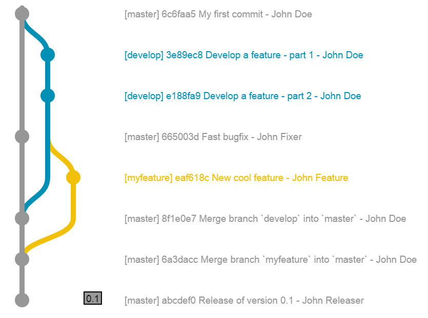
The gray line is the master branch (now called main^[7]), and the blue and yellow lines are copies (develop and myfeature) that branched off at different points, were modified, and then were merged back into master. You can have dozens of branches running in parallel at larger companies, which is essential for letting teams of developers work on the same codebase simultaneously. The only branch the customer ever sees, though, is main.

The actual code behind using Git is straightforward. Below are some commands in bash in the Mac Terminal, where we:

Switch from whatever branch we were on onto the main branch
Create a new branch, DS-123-Add-outlier-check^[8], that is a copy of main
Push the branch from our local computer and onto GitHub

bash

git checkout main
git checkout -b DS-123-Add-outlier-check
git push --set-upstream origin DS-123-Add-outlier-check

Now, on our new branch, we’re free to make whatever changes to the code we’d like. Let’s say we modify preprocessor.py by adding a step that removes outliers. When we want to save our changes, we type the following into the Terminal.

bash

git add preprocessor.py
git commit -m "Add outlier check"
git push

These steps are only reflected on DS-123-Add-outlier-check, not main. This lets us prepare the code until it’s ready to be pushed to main.

And if we broke something and want to revert to an old commit? We checkout to that commit using its hash, tell Git to ignore the commit with errors, then push our changes to the branch.

bash

git checkout abc123  # go to old checkpoint
git revert bad456    # "delete" the bad checkpoint
git push             # update the branch

Object-oriented programming

As the amount of code in a project grows, it typically follows this pattern of increasing organization:

Scripts with raw commands one after the other
Commands grouped into functions
Functions grouped into classes
Classes grouped into modules

Production-level Python is best at the fourth level of organization, where code can easily be added, modified, and reused across contexts. A team’s code will typically be organized into modules based on company products (e.g. “data quality alerts,” “price forecasters,” “customer churn predictors”), which in turn contain classes with collections of functions that work together. Below is a brief example of a class called Student.

Python

class Student:
    def __init__(self, name, grade):
        self.name = name
        self.grade = grade

    def introduce(self):
        print(f"{self.name} is in grade {self.grade}")

john = Student("John", 3)
mary = Student("Mary", 5)

john.introduce()  # 'John is in grade 3'
mary.introduce()  # 'Mary is in grade 5'

Classes may be stored in .py files with the same name, grouped into folders with similar classes. The module is the directory containing all the folders. We can have a data_processing module, for example, with a directory structure like this^[9]:

data_processing
|   init.py
|   cleaners
|   |   init.py
|   |   data_cleaner.py
|   visualizers
|   |   init.py
|   |   error_logger.py
|   |   dashboarder.py
|   services
|   |   init.py
|   |   data_loader.py
|   |   database_writer.py

In the cleaners subdirectory, data_cleaner.py contains a class, DataCleaner, with methods for cleaning data. The first 60 lines of data_cleaner.py might look something like this:

Python

import logging
import pandas as pd
from typing import Optional, List

from ..services import DataLoader

# Global variables
N_SD_THRESH = 5  # N std devs from mean where value flagged as outlier
MAX_TRIES = 3    # N tries before function stops


class DataCleaner:
    """
    | Functions for cleaning data
    """
    def __init__(self, max_tries: int = MAX_TRIES):
        self.max_tries = MAX_TRIES
        self.dl = DataLoader()

    def remove_outliers(self,
                        df: pd.DataFrame,
                        cols: Optional[List[str]] = None,
                        n_sd_thresh: int = N_SD_THRESH) -> pd.DataFrame:
        """
        | Remove values > n_sd_thresh from mean of cols in df.
        | If cols not specified, all columns in df are processed.
        |
        | -------------------------------------------------------
        | Parameters
        | ----------
        |  df : pd.DataFrame
        |    The data
        |
        |  cols : list or None
        |    Columns to remove outliers from
        |
        |  n_sd_thresh : int
        |    Number of standard deviations from mean above/below
        |    which a row is excluded
        |
        |
        | Returns
        | -------
        |  pd.DataFrame
        |    Original df with rows with outliers removed
        """
        cols_to_check = cols if cols is not None else list(df)

        bad_rows = set()
        for col in cols_to_check:
            bad_rows.update(self._find_outliers(df[col], n_sd_thresh))

        df_filt = df[~df.index.isin(bad_rows)].reset_index(drop=True)

        if df_filt.empty:
            logging.warning("df has no rows without outliers")

        return df_filt

This code block is quite a bit longer than the others, and it doesn’t even include the helper function _find_outliers or code that calls DataLoader. For production-level coding, there’s a lot more architecture you need to build around your core functions to ensure that your code:

Can be read and modified by others, not just you
Is modular enough to be used in pipelines and multiple contexts
Doesn’t grind those pipelines to a halt if it gets some unexpected input

The code above has a detailed docstring, type hints, argument defaults set to global variables at the top of the file, and a warning log for unexpected behavior. These add-ons help explain what our code is doing to other developers $-$ as well as to ourselves! As a further precaution, we could incorporate error-handling for when an argument of the wrong datatype is passed in, which would otherwise cause our script to fail.

Virtual environments

Unless our code is very simple, we’ll need to import external libraries (like pandas and numpy). These external dependencies, as Bill Sourour puts it, “are the devil.” Code is constantly evolving, and sometimes a script you wrote a year ago no longer works when it uses the latest versions of its dependencies. Python 3 is famously backward incompatible with Python 2, for example, and pandas v1.0 deprecated or removed several Series and DataFrame operations.

One way to protect against changing dependencies is to take a “snapshot” of your project’s external libraries $-$ and their exact version numbers. We can then create a virtual environment that lets us recreate what the “external code world” looked like when you created your project and everything ran correctly.

In the Terminal, we can use Python’s built-in virtualenv module to create a virtual environment. Here, we create one called venv.

bash

python -m virtualenv venv

We can then enter this virtual environment by typing the code below:

bash

source venv/bin/activate

Our new environment has none of the libraries our global environment has. For example, even if you installed scikit-learn before creating the virtual environment, scikit-learn doesn’t exist in venv. We’re starting from a clean slate whenever we create a new environment! We’ll therefore need to (re)install each library we need for our project inside venv. We can specify version numbers with the <package>==<version> syntax if needed.

bash

pip install pymongo
pip install scikit-learn==0.24

Once our virtual environment has all packages downloaded and you’ve verified your application works, we can save all packages and their version numbers to a file, requirements.txt, with the following command. pip freeze returns all downloaded libraries, and the > operator pipes that output into a file instead of printing it on the screen.

bash

pip freeze > requirements.txt

In the future, to ensure our project works as expected, we can then create a new virtual environment and install the exact versions of all dependencies with pip install -r requirements.txt. This works great for relatively small-scale work, but if you’re deploying a package, e.g. to PyPI itself for others to download, you’ll want to dig into more advanced setuptools methods.

Writing tests

When we write a function, the code should do what we want it to do. But to take it a step further, our code should also not do anything else. While this might seem obvious, that extra step requires a lot of additional architecture in our code. Here’s a simple example:

Python

def multiply(a, b):
    """Multiply two numbers!"""
    return a * b

# Expected behavior - great!
multiply(1, 2)  # 2

# Unexpected - uh oh...
multiply([1], 2)  # [1, 1]
multiply('1', 2)  # '11'

Our multiply function veers into string and list concatenation when it gets a non-number input. This probably isn’t what we want!

It’s easy to dismiss these examples as irrelevant, but this could easily happen if multiply was deep in a pipeline, taking in the outputs of a previous function, which took in the outputs of some function before that. We could have a find_anomalies function, for example, that returned 0 if there were no anomalies, and a list of values if there were anomalies. (Don’t do this $-$ try to always have the same datatype returned from a function.) If multiply took the outputs of find_anomalies, we’d get drastically different results based on what find_anomalies returns, which would likely break our pipeline.

Python

def find_anomalies(values):
    above_5 = [val for val in values if val > 5]
    if len(above_5) > 0:
        return above_5
    else:
        return 0  # (don't do this)

# Outcomes differ drastically
multiply(find_anomalies([1, 2]), 2)    # 0
multiply(find_anomalies([10, 20]), 2)  # [10, 20, 10, 20]

The way to catch these issues, and to learn how to write better code in general, is to write tests. A test is basically what it sounds like: there’s a “right answer” output for some input, and you check whether your code produces that correct output. Tests vary in how much of the code they check: you can write tests for the entire application, a subset of components, or individual functions. I’ll briefly cover the last type, unit tests, below.

A good set of unit tests for a function will cover three types of inputs: good, special, and bad. A good input is what it sounds like: the input this function is intended to receive, like integers or floats for our multiply function. A special input is an “edge case,” perhaps something that triggers internal logic to deliver a different output. Finally, a bad input is one that our function can’t handle whatsoever $-$ our function should fail.

Let’s rewrite multiply^[10] and then then write some tests. Lines 8-12, about 83% of our function, are now purely devoted to making sure multiply doesn’t break. These lines really do the trick $-$ we end up not needing to write tests for bad inputs, as we can’t throw anything at multiply that causes it to break. Believe me, I’ve tried.

Python

import logging
from typing import Union

def multiply(a: Union[int, float],
             b: Union[int, float]) -> Union[int, float, type(None)]:
    """Multiply two numbers. If non-numbers are passed in,
        returns None."""
    for name, val in locals().items():
        if not isinstance(val, (int, float)):
            logging.error(f"Non-numeric input received: {name} is" +
                          f"type {type(val)}. Returning None.")
            return None
    return a * b

We can then use the pytest library to write our tests. The first step is to clearly define our types of inputs and their expected outputs. I like to use nested dictionaries, where the top layer is our test case (e.g. int-int, meaning both a and b are integers), and the inner layer is a dictionary of our argument names and their values. We can then use **kwarg notation to unpack the dictionary into the function we’re testing.^[11]

Python

import pytest
from src import multiply

class TestMultiply:

    GOOD_INPUTS = {"int-int": {"a": 1, "b": 0},
                   "int-float": {"a": 1, "b": 0.0},
                   "float-int": {"a": 1.0, "b": 0},
                   "float-float": {"a": 1.0, "b": 0.0}
                  }

    SPECIAL_INPUTS = {'list': {'a': [1, 2], 'b': 3},
                      'str': {'a': 1, 'b': 'abc'}}

    GOOD_OUTPUT = 0.0
    SPECIAL_OUTPUT = None

    def test_return_number(self):
        for name, kwargs in self.GOOD_INPUTS.items():
            actual = multiply(**kwargs)
            assert actual == self.GOOD_OUTPUT, (
                f"Got {actual} for {name} case; " +
                f"expected {self.GOOD_OUTPUT}")

    def test_return_none(self):
        for name, kwargs in self.SPECIAL_INPUTS.items():
            actual = multiply(**kwargs)
            assert actual == self.SPECIAL_OUTPUT, (
                f"Got {actual} for {name} case; " +
                f"expected {self.SPECIAL_OUTPUT}")

The actual testing happens in the assert statements, which are silent if the first argument returns True, and raise an AssertionError with the text in the second argument if False. It’s good to be detailed in the assertion string if your test fails, as that’ll help you pinpoint the error.

I recommend structuring your tests in a directory that mirrors the structure of your repository, like below.

src
|   custom_math
|   |   easy
|   |   |   add.py
|   |   |   subtract.py
|   |   hard
|   |   |   multiply.py
|   |   |   divide.py
|   tests
|   |   test_easy
|   |   |   test_add.py
|   |   |   test_subtract.py
|   |   test_hard
|   |   |   test_multiply.py
|   |   |   test_divide.py

You can then navigate to the root folder of your project (src above), then just type pytest tests to run all tests. Note that the functions, classes, and filenames need to either start or end with test for pytest to recognize them as tests.

Once you’ve got this down, take your tests to the next level by mocking dependent functions and asserting about exceptions.

Concluding thoughts

As with the statistics post, it’s hard not to write a textbook when it comes to useful software engineering practices for data science. When I started transitioning into data science, my greatest knowledge gap was by far the engineering. There’s just so much besides the actual analytics when it comes to building the machine. How do you create an application rather than a one-off script? How do you sustainably write thousands of lines of code, or work with others on a codebase of potentially millions of lines? The concepts in this post, from managing dependencies to writing resilient code, should help fill this knowledge gap. If you’re itching for more, check out Python decorators, creating your own API endpoints, Docker containerization, and application hosting services like Heroku.

In the next and final post in this series, we’ll turn to the people in data science: stakeholders and yourself. It’s great if you have the most cutting-edge analytics and an infinitely scalable application, but how do you get decision-makers to care? What questions deliver business value versus “nice to know” tidbits? At the other end, how do you stay motivated and relevant in a field that’s constantly changing? Stay tuned to find out.

Best,
Matt

Footnotes

1. The code around your code

This is aimed at me as much as at anyone else. In grad school, I had R scripts that were hundreds of lines long, and rerunning them to process data differently always felt like performing surgery. It shouldn’t be that way! Looking back, it’s amazing how much easier the Ph.D. would have been with some basic software engineering and project management best practices in place. Maybe for the next doctorate…

2. SQL

A popular alternative to relational databases is NoSQL, or non-relational databases (a.k.a. “Not Only SQL.”) In contrast to tables with strictly defined relationships, NoSQL databases like MongoDB allow much more flexibility in how data are stored. You can store arrays or nested dictionaries, or even add fields to documents (“tables”) in the database on the fly. A major disadvantage to this flexibility, however, is that complex queries are less flexible, especially joining data from separate documents together. While NoSQL databases are popular, traditional relational databases are still more common so I’ll focus on them here.

3. SQL

Searching, inserting, and deleting records in a properly-indexed database is expected to scale at $O(\log{n})$. This means that for every order of magnitude, traversing the data requires only one additional step! I find this mind-boggling.

4. SQL

In the research for this post, I stumbled across this (somewhat controversial) SQL Style Guide. It was an interesting read, and I decided to adopt some of the layout tips for the SQL examples in this post. The main thing I took away was having a blank “river” down the middle of your code, with SQL keywords on the left and the rest of the code on the right $-$ it makes it really easy to quickly scan what the query is doing. If I don’t find an easy way to auto-format the code this way, though, I doubt I’ll stick with it for quick analyses.

5. SQL

If this actually happens to you, hopefully your company’s engineering team regularly backs up the databases and can roll back to an earlier version. If they don’t, and you accidentally delete all your company’s data, then Quora recommends you resign and find a company with better engineering practices!

6. Interacting with APIs

APIs and SQL go hand-in-hand, actually. When you request data from an API, your request is most likely converted to a SQL query that is then executed on a database.

7. Version control

In October 2020, GitHub renamed the default branch for new repositories from master to main to remove unnecessary references to slavery.

8. Version control

A best practice naming convention for Git branches is to refer to them by their JIRA ticket ID. If your company integrates Git with JIRA, other developers will see whether the branch is in development, has an active pull request, or has been merged into main. An even better (“best”-er?) practice is to include in the branch name whether it is a hotfix, support request, part of the roadmap, etc.

9. Object-oriented programming

The init.py files allow for classes to be imported from outside their directory. This is what allows from ..services import DataLoader in the next code block to work. Similarly, if you have your data_processing module installed, you can be in any script and load DataLoader by typing:

# With init files
from data_processing import DataLoader

Without the init files, you would need to type:

# Without init files
from data_processing.services.data_loader import DataLoader

Not only is this far less convenient, it also runs the risk of external scripts breaking if you decide to rearrange the directories inside the data_processing module. You can read more about init.py files here.

10. Writing tests

If we really want to be thorough, we should break out a helper function to check the inputs to multiply. This keeps our functions focused on as few tasks as possible, making writing tests and debugging easier. Here’s what that would look like:

# Main function
def multiply(a: Union[int, float],
             b: Union[int, float]) -> Union[int, float, type(None)]:
    """Multiply two numbers. If non-numbers are passed in,
        returns None."""
    if not _multiply_inputs_valid(a, b):
        return None
    return a * b

# Helper function
def _multiply_inputs_valid(a, b) -> bool:
    """Check whether inputs are int or float"""
    for name, val in locals().items():
        if not isinstance(val, (int, float)):
            logging.error(f"Non-numeric input received: " +
                          f"{name} is type {type(val)}.")
            return False
    return True

11. Writing tests

I find unpacking tuples and dictionaries makes writing tests a lot more fun. Here’s the notation with and without unpacking.

input_tuple = (1, 0)
input_dict = {'a': 1, 'b': 0}

# Without unpacking
multiply(input_tuple[0], input_tuple[1])
multiply(input_dict['a'], input_dict['b'])

# With unpacking
multiply(*input_tuple)
multiply(**input_dict)

Written on December 30, 2020

How to enter data science 4. The engineering

The code around your code

Accessing data

SQL

Interacting with APIs

Web scraping

Version control

Object-oriented programming

Virtual environments

Writing tests

Concluding thoughts

Footnotes

1. The code around your code

2. SQL

3. SQL

4. SQL

5. SQL

6. Interacting with APIs

7. Version control

8. Version control

9. Object-oriented programming

10. Writing tests

11. Writing tests

How to enter data science
4. The engineering